Before the end of the last year I went to see a movie made by one of my favourite movie directors, Damien Chazelle. The movie is called First Man and it tells the story of the journey of the first man on the Moon. I am also a bit of a space nerd, so my expectations were sky high. I was happy to find out the movie delivered on its promise.
What I liked about it the most was that it showed the [human] sacrifice that had to be made in order to achieve, what has arguably been one of the biggest achievements of humankind to date. Many lives were ruined [and lost] in the pursuit of greatness and place in the history. Astronauts would compete with each other for the spots on the spaceships in spite of knowing they might not return back to Earth at all. Besides every [technological] achievement there is a price to pay. Some are high, others are higher. This was the golden era of space exploration, the era when the geopolitical tensions around the world were immense.
Some people might not appreciate how much software engineering went into getting people to space and ultimately to the Moon. But with a little bit of exaggeration, you could think of Apollo Program as finding a way to “shoot” huge edge computers carrying people to space and deliver them safely to the Moon and back. In today’s hyper computing era with so many edge computers orbiting the earth it might not seem like that big of a deal, but given the state of the computing in 60s-70s in 20th century, getting people to the Moon on these “computers” was a huge task!
Watching the movie made me remember my time at university when I learnt about something that was fundamental for the success of Apollo 11 mission: Kalman filter.
I’m not going to talk too much about Kalman filter in this post. There is plenty of great material to be found on the web if you want to learn about it. In particular, I really liked this post by Tim Babb who explains the Kalman filter so well that I could not possibly do a better job even if I tried. Go ahead and read it. The math can seem a bit daunting to some, but even if you skip the math formulas I reckon you can still get a basic intuition behind it.
Another great source [if not slightly more technical] for building the intuition behind how Kalman Filter works is this post by David Khudaverdyan. It even contains a short code snippet in Matlab!
Discovery of Kalman Filter
What I would like to to talk about in this post is something I discovered after I got back home from the cinema when I started doing a bit of research about the use of Kalman filter in Apollo missions. Don’t ask why! Apparently, NASA keep a publicly available memo of the events that led to development of the Kalman filter for the Apollo program: “Discovery of the Kalman filter as a practical tool for aerospace and industry “.
You can find the link to the full memo here. I encourage you to read it because it’s pretty amazing. But if you are too busy, just carry on reading – I took the liberty of taking some screenshots from it and posting them here with my comments. Reading the memo led me to decision to hack on the Kalman filter, but more about that later.
Problem
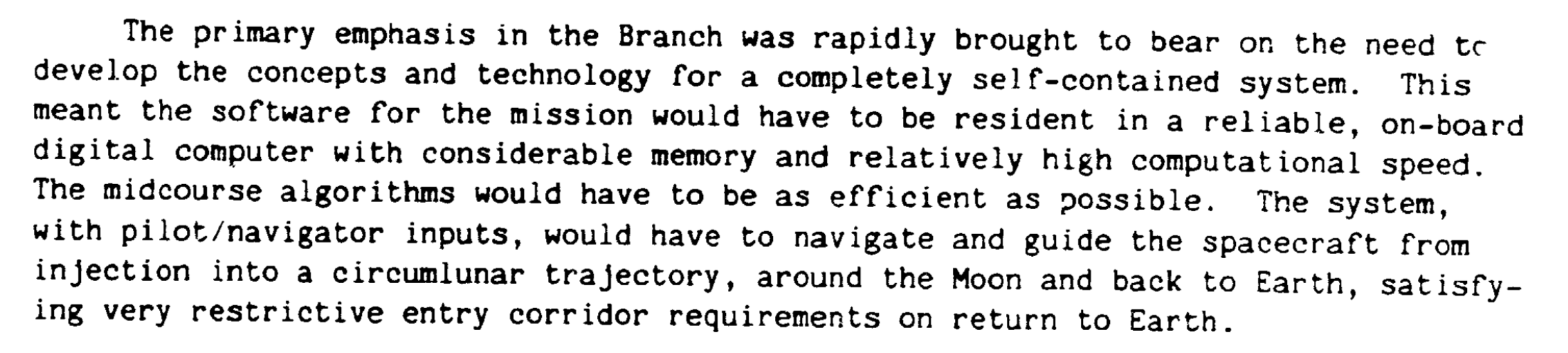
Let’s start by framing the problem NASA engineers and scientists were trying to solve. You have a rocket, which carries a few people and some cargo. The spaceship has a lot of sensors on it which feed data to the computers onboard [and to the mission control back on Earth]. The sensors are not 100% accurate because of the omnipresent measurement noise. Some things you can’t measure directly without damaging the sensors, so you need to estimate them. Some sensors might not provide any measurements at all during some periods of time and some will completely fail. Your goal is to get some people to the Moon and back. In other words: all you have is a bunch of noisy sensors and primitive (in a sense of today’s time) computers and you need to build a self-flying spacecraft:
NASA Apollo program team
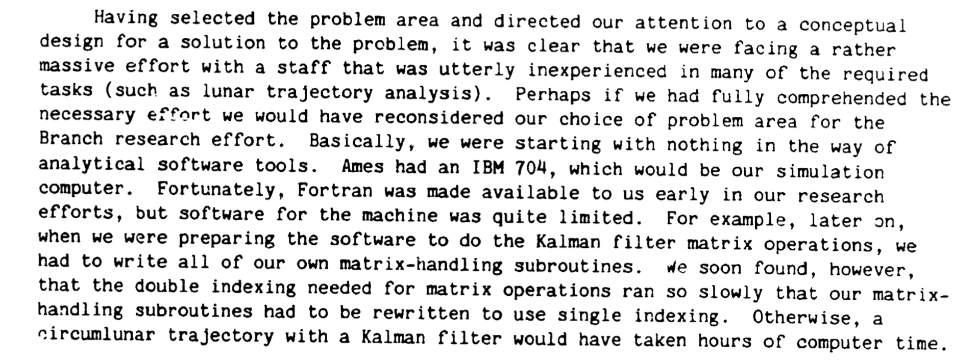
The NASA team behind Apollo Program seemed like a small startup: you’ve got a bunch of people, some of whom are software developers, who want to achieve something great whilst very few of them know how to go about it or if it’s even possible. Luckily, as the memo says, they’ve got this amazing pogramming language available at their disposal to make things fast(er): “Fortunately, Fortran was made available to us in early in our research efforts…”:
No Kalman, more cry
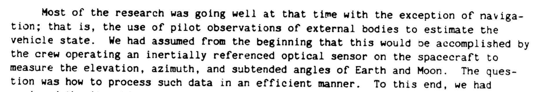
Everything was going sort of ok until the team started facing the main problem: they needed to predict the trajectory of the spacecraft so they could correct it taking into account the measurements [and their noise] as well as the occasional lack of them, so you can get the spacecraft safely to the Moon. And it had to be extremely efficient given the computing resources at their disposal. which they refer to in the memo as “digital computers”:
Rudolf Kalman
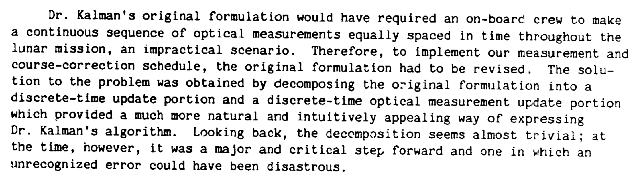
This is where Rudolf Kalman enters the picture. He developed a new kind of dynamical state estimator/filter which seemed like it could be of interest to the Apollo team. But as it always happens, the problem with cutting edge research is that at the beginning it’s almost always impractical for real life tasks, so the Apollo team had to put in a lot of effort to make it usable:
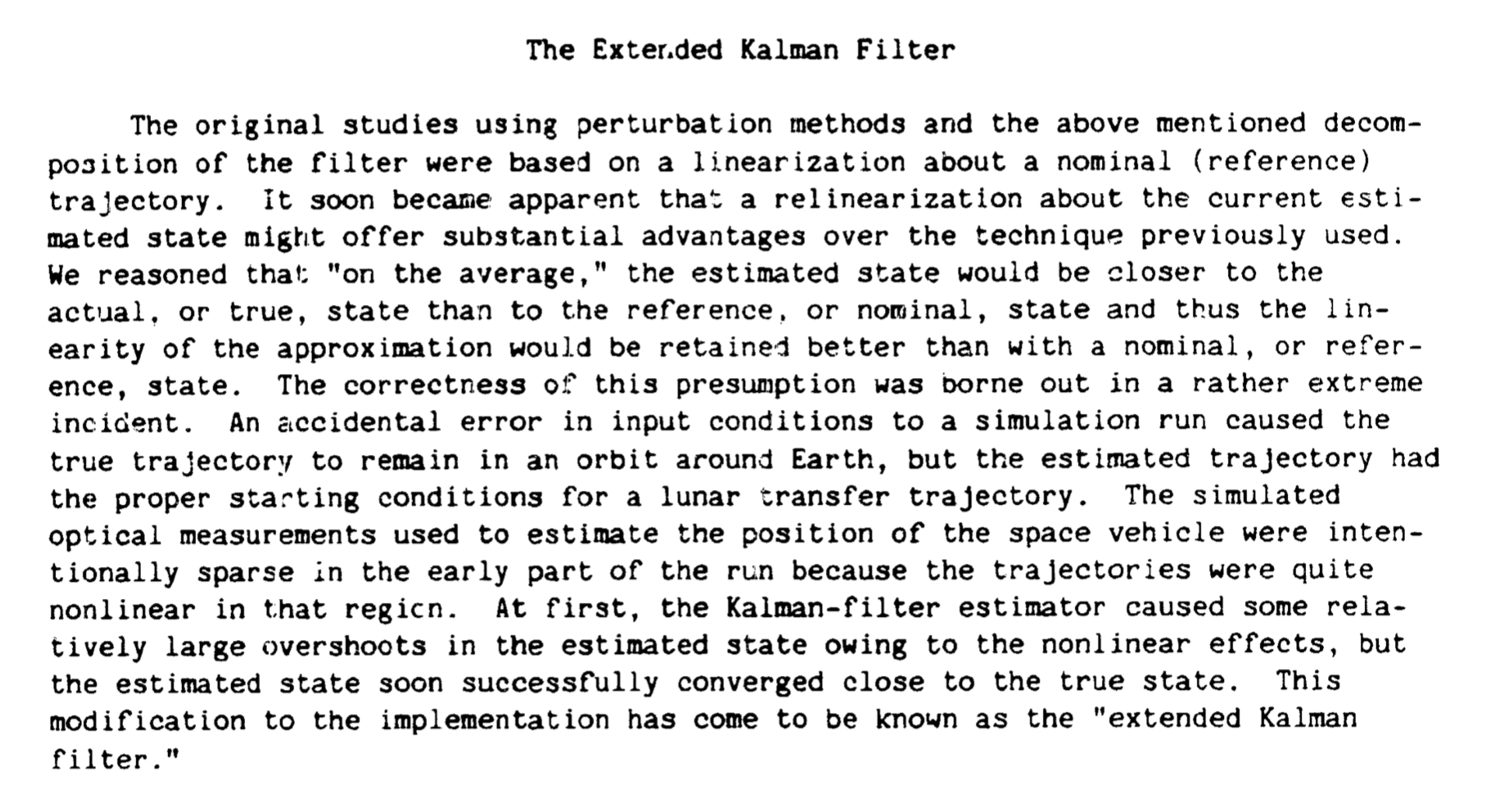
Furthermore, the original Kalman filter was designed to work with linear estimation problems. It turns out this is often ok for many non-linear problems, too, but sending people to space did not fall into this category. Son the NASA team came up with a new variant of the Kalman filter which would accommodate the non-linearities . To honour the creator of the original filter they decided to call it Extended Kalman Filter:
Development
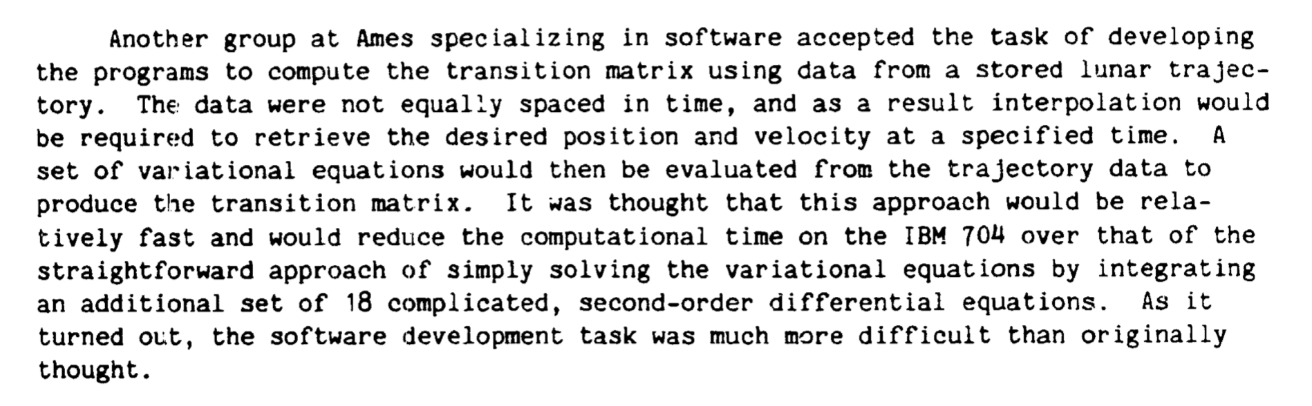
Now that the theoretical work was done, the filter had to be programmed. NASA did not seem to be much different from modern day software companies when it came to [under]estimating the effort to deliver the implementation of the solution designed by researchers:
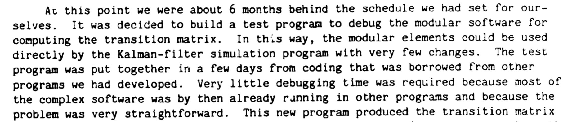
As always when working with cutting edge tech, you inevitably end up facing a lot of [interesting] problems no one has faced before. This was probably the bread and butter for the Apollo team throughout the whole program. Luckily, if you design your code well, sharing the code from other projects makes your life easier, so ”…very little debugging time was required…”:
But bugs always crawl into your software. Luckily, the team discovered them during intensive testing on the simulator (hello integration testing!):


Fixing the bugs was just a small part of the number of issues the team had encountered on their way to making the program which could be safely used on the spaceships. There were problems with numerical stability or the lack of memory to calculate various matrix operations without compromising on the precision and accuracy which were paramount for the mission. The memo describes some fascinating stories behind the solutions to some of the problems no one had ever faced before.
Delivery
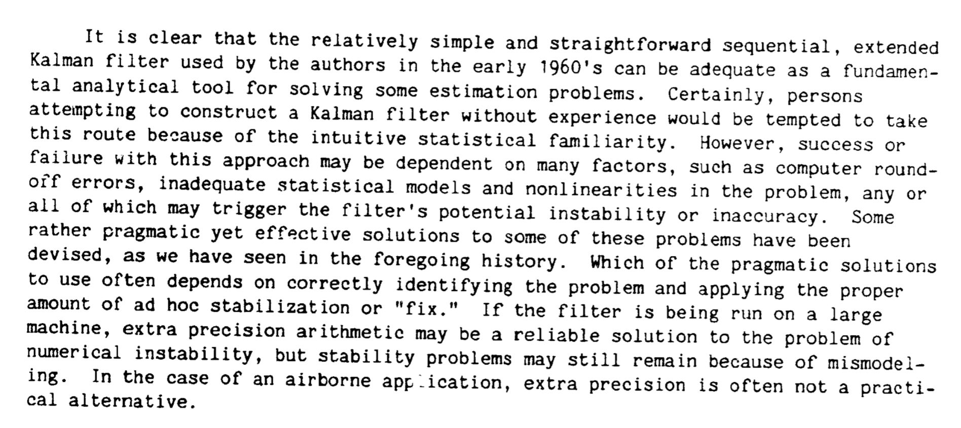
Eventually the software was delivered and it was quite a feat of mathematics, science and software engineering. What I loved about the closing remarks was the following mention:
“Some rather pragmatic, yet effective solutions to some of the problems have been devised….which of these pragmatic solutions to use often depends on correctly identifying the problem and applying the proper amount of ad hoc stabilisation or “fix” “.
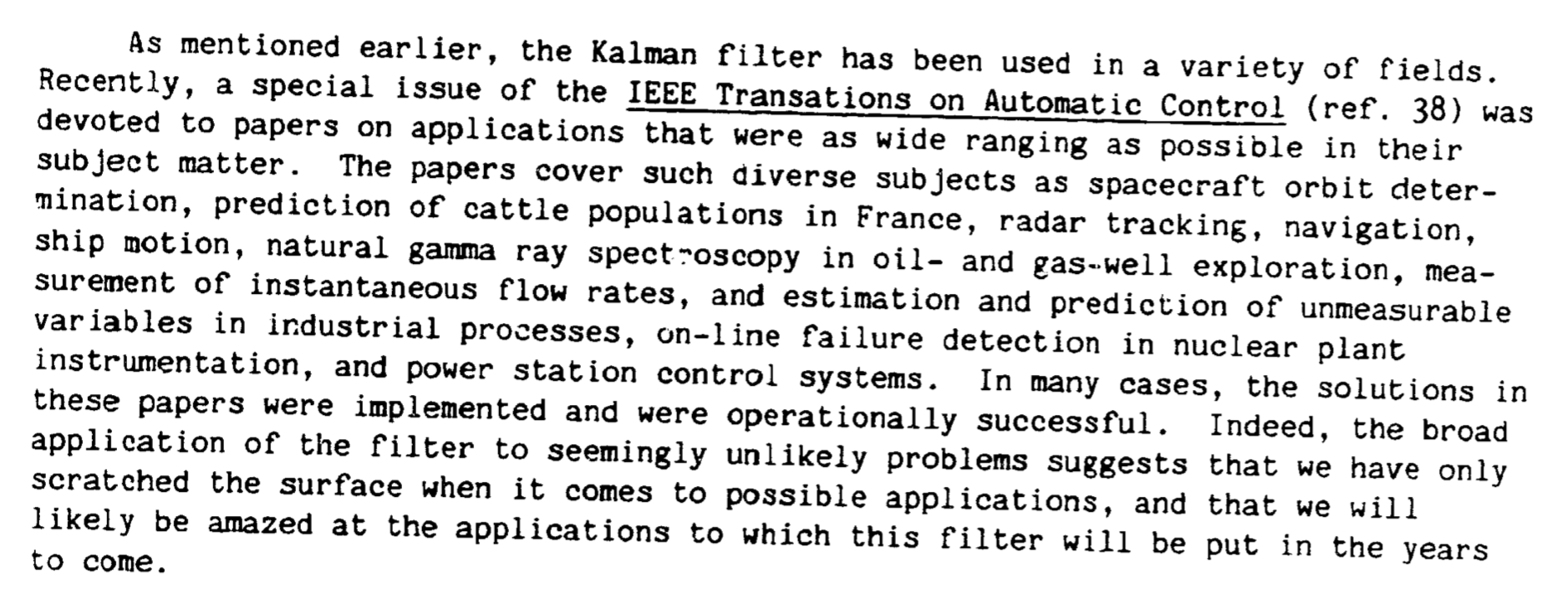
The invention of Kalman filter sparked a lot of innovation during and after the Apollo program which led to creating of many new variants of it. Kalman filter ended up being used in great many fields beyond aeronautics:
go-estimate: Go package for filtering and state estimation
After I finished reading the NASA memo I decided to hack on some Kalman filter algorithms for fun. I just finished my last freelance gig and had no other interesting side project to pursue, so this felt like a perfect way to both revisit the old and picking up some new knowledge.
My original plan was to hack only on the original [a.k.a. linear] Kalman Filter, but the deeper I dived in the more fun I had and the more Kalman variants I ended up hacking on. At some point I started looking into some other filtering algorithms, such as particle filter. Eventually I made a decision to turn the whole effort into a simple Go package called go-estimate.
The package is available on GitHub. It currently implements several variants of Kalman Filter as well as Bootstrap Filter which is a specific type of the particle filter mentioned earlier.
Now, if you know a bit about filtering and state estimators or if you’ve read Tim Babb’s blog post you would know the filter works in two steps:
-
Predict: based on the [ideal] model dynamics, the filter predicts the next internal state of the system. The next state is not accurate as it contains nonlinearities such as noise as well as the nonlinearities propagated to it from the previous state. This has an effect on the predicted state (and its covariance matrix) being a bit off the nominal (i.e. idealised) model
-
Update: int this step the filter corrects the internal state (and its covariance matrix) predicted in the previous step using the measurement provided by external sensor(s). The end result is, the internal state being closer to the nominal state, but ideally not exactly the same, since you are attempting to model the reality, not the ideal model.
The above mental model of how the filter works is reflected in the package design. I think the current abstractions might be just about ok to continue to build on further:
// Filter is a dynamical system filter.
type Filter interface {
        // Predict estimates the next internal state of the system
        Predict(mat.Vector, mat.Vector) (Estimate, error)
        // Update updates the system state based on external measurement
        Update(mat.Vector, mat.Vector, mat.Vector) (Estimate, error)
}
The filter interface only requires to implement Predict() and Update() functions. In order to implement either of them the filter needs to embed a model which provides functions that allow to propagate the internal state and observe the external state of the system. Putting it all together the whole system looks something like this:
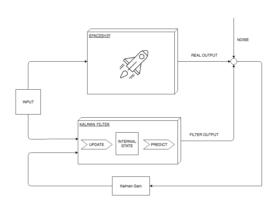
This diagram may confuse you a bit since I said before that the filter first predicts and then updates the internal state. So let me make things a bit clearer. Kalman filter is a recursive state estimator: it predicts state at time \(k+1\) from state at time \(k\) where the state \(k\) is the previously updated (corrected) state. Now when the filter is created you need to “estimate” the updated (corrected) state from which the next state is predicted: this is called initial condition of the filter.
The model mentioned earlier is supposed to mathematically model the system whose state you are trying to estimate.The Model interface is pretty simple. You need to propagate the state at time \(k\) to state at time \(k+1\)and then observe the output of the system produced at time \(k+1\). The Model interface is designed to work with vectors since both the internal and external states are often multidimensional.
// Model is a model of a dynamical system
type Model interface {
        // Propagator is system propagator
        Propagator
        // Observer is system observer
        Observer
        // Dims returns input and output dimensions of the model
        Dims() (in int, out int)
}

// Propagator propagates internal state of the system to the next step
type Propagator interface {
        // Propagate propagates internal state of the system to the next step
        Propagate(mat.Vector, mat.Vector, mat.Vector) (mat.Vector, error)
}

// Observer observes external state (output) of the system
type Observer interface {
        // Observe observes external state of the system
        Observe(mat.Vector, mat.Vector, mat.Vector) (mat.Vector, error)
}
Finally, creating a particular type of filter is done by calling New function of the chosen filter package. See the example of how to create [Linear] Kalman Filter, which is implemented in kf package:
// create Kalman Filter
f, err := kf.New(model, initCond, stateNoise, measNoise)
if err != nil {
    log.Fatalf("Failed to create KF filter: %v", err)
}
Please check out the godoc for the full API documentation and open an issue and/or pull request if you find some mistake in the docs.
There are a few sample programs available in the examples GitHub repo, so go check them out. In particular, I’d recommend you to play a bit with the ones which use the wonderful gocv library. Take for example the short gif below which demonstrates the usage of the bootstrap filter:
The green mark in the GIF represents the nominal trajectory of the spaceship i.e. the model trajectory (it needs no correcting). The mark represents the corrected trajectory of the spaceship as produced by the filter. Finally, the red mark, which as you can see fluctuates a lot around the model trajectory, represents the noisy measurements as returned by hypothetical sensors. The tiny white dots which surround both the nominal and corrected trajectory marks are the filter particles which are used by filter to calculate the state update. The simulation example uses 100 particles which give pretty good results.
Conclusion
Working on go-estimate was a lot of fun. I wish I had this package available for some of the projects I worked on for Intel last year. I’m pretty sure It would have helped me to improve the results of at least the car tracking algorithms I hacked on. Kalman filter is indeed used in many navigation and position tracking algorithms, so it would have made for a natural fit for the problem of car tracking. This is the case with self-driving cars or robots which use some variants of state estimators for localisation and mapping, so I think it’s worth learning about them.
Besides, state estimators like Kalman filter are already omnipresent in our lives without our knowing about it: clear sign the technology works pretty well. Filter usage will become even more prevalent the more sensors we will have been deployed in the future. These sensors will inevitably return noisy measurements which will have to be corrected.
I hope you enjoyed this blog post as much as I enjoyed writing it. If you have some cool use case for using some filters, please leave a comment, I would love to hear about it. Don’t hestitate to open an issue or PR on GitHub. Until next time!