Couple of months ago I came across a type of Artificial Neural Network I knew very little about: Self-organizing map (SOM). I vaguely remembered the term from my university studies. We scratched upon it when we were learning about data clustering algorithms. So when I re-discovered it again, my knowledge of it was very basic, almost non-existent. It felt like a great opportunity to learn something new and interesting, so I rolled up my sleeves, dived into reading and hacking.
In this blog post I will discuss only the most important and interestng features of SOM. Furthermore, as the title of this post suggests, I will introduce my implementation of SOM in Go programming language called gosom. If you find any mistakes in this post, please don’t hesitate to leave a comment below or open an issue or PR on Github. I will be more than happy to learn from you and address any inaccuracies in the text. Let’s get started!
Motivation
Self-organizing maps, as the name suggests, deal with the problem of self-organization. The concept of self-organization itself on its own is a very fascinating one
“Self-organization is a process where some form of overall order arises from local interactions between parts of an initially disordered system….the process is spontaneous, not needing control by any external agent” – Wikipedia
If you know a little bit about physics, this should feel familiar to you. The physical world often seems like an “unordered chaos” which on the outside functions in orderly fashion defined by interactions between its elements (atoms, humans, animals etc.). It should be no surprise that some scientists expected our brains to behave in a similar way.
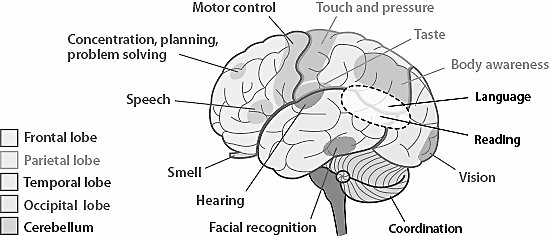
The idea that brain neurons are organized in a way that enables it to react to external inputs faster seems plausible: the closer the neurons are, the less energy they need to communicate, the faster their response. We now know that certain regions of brain do respond in a similar way to specific kind of information, but how do we model this behaviour mathematically? Enter Self-organizing maps!
Introduction
SOM is a special kind of ANN (Artificial Neural Network) originally created by Teuovo Kohonen and thus is often referred to as Kohonen map. Unlike other ANNs which try to model brain memory or information recognition, SOM focuses on different aspects. Its main goal is to model brain topography. SOM tries to create a topographic map of brain. In order to do this it needs to figure out how the incoming information is mapped into different neurons in the brain.
Brain maps similar information to groups of dedicated regions of neurons. Different pieces of information are stored in dedicated areas of brain: internal representations of information in brain are organised spatially. SOM tries to model this spatial representation: you throw some data onto SOM and it will try to organize it based on its underlying features and thus generate a map of brain based on what information is map to what neurons.
Representation
SOM representation is different from other neural networks. SOM has one input layer and one output layer: there are no hidden layers. All the neurons in the input layer are connected to all the neurons in the output layer. Input layer feeds incoming information [represented as arbitrary multidimensional vectors \(x_{i}\)] to output layer neurons. Each output neuron has a weights vector \(m_{i}\) associated with it. These weights vectors have the same dimension as the input vectors and are often referred to as model or codebook vectors. The codebook vectors are adjusted during training so that they are as close to the input vectors as possible whilst preserving topographic properties of the input data. We will look into how this is done in more detail in the paragraph about SOM training.
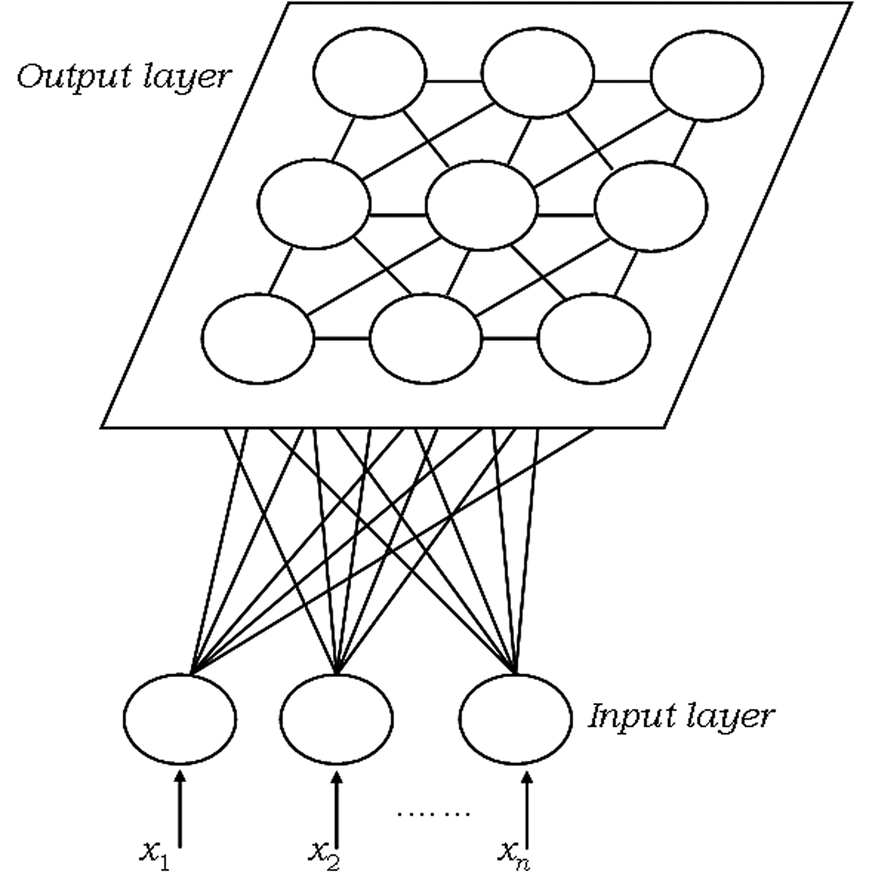
Note how the output neurons are placed on a 2D plane. In fact, SOM can be used to map the input data to 1D (neurons are aligned in line) or 3D (neurons are arranged in a cube or a toroid) maps, too. In this post we will only talk about 2D maps, which are easier to understand and also most widely used in practice. The output neuron map shown above represents [after the SOM has been trained] the topographic map of input data patterns. Each area of the output neuron map is sensitive to different data patterns.
Based on this representation we can assume that each output neuron in SOM has two properties:
- topography: position on the outut map (map coordinates)
- data: codebook vector of the same dimension as input data
SOM feeds input data into output neurons and adjusts the codebook vectors so that the output neurons which are closer together on the output map are sensitive to similar input data patterns: neurons which are close to each other fire together. This was a bit mouthful I know, but we will see in the next parapgraph that in practice it is not as complex as it sounds. Let’s have a look at the training algorithm which will help us understand SOM better.
Training
SOM is no different from other ANNs in a way that it has to be trained first before it can be useful. SOM is trained using unsupervised learning. In particular, SOM implements a specific type of unsupervised learning called Compettive learning. In competitive learning all the output neurons compete with each other for the the right to respond when presented a new input data sample. The winner takes it all. Usually the competition is based on how close the weights of the output neuron are to the presented input data.
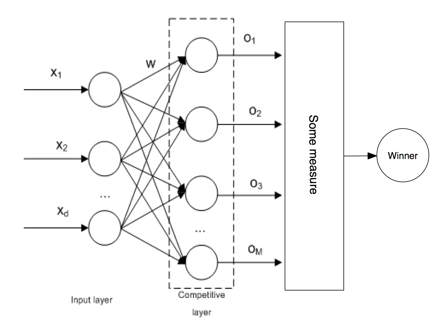
In case of SOM, the criterion for winning is usually Euclidean distance, however new alternative measures arose in recent research which can achieve better results for different kind of input data. The winning neuron codebook vector is updated in a way that pulls it closer to the presented data:
$$ w(t+1) = w(t) + \alpha(t) . (x(t) - w(t)) $$
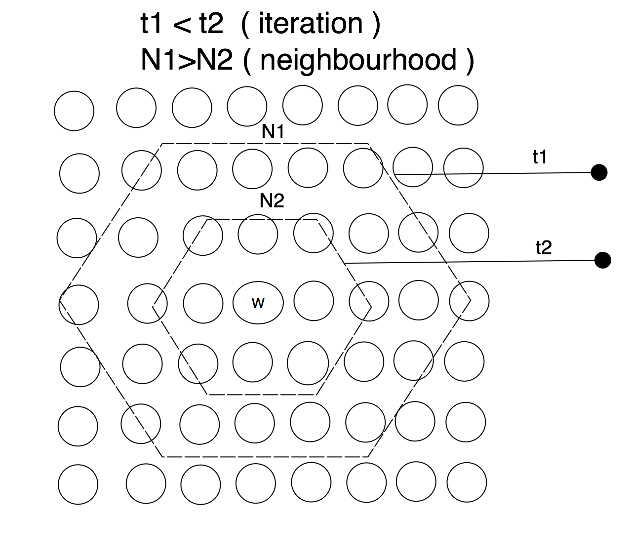
SOM takes the concept of competittve learning even further. Not only does the winning neuron gets to update its codebook vector, but so do all the neurons in its close topological neighbourhoodp. SOM neurons are thus selectively tuned: only the ones which are close to winner are updated. SOM learning is different from backpropagation where ALL [hidden and output] neurons receive the updates.
The winning neuron’s topological neighbourhood starts quite large at the beginning of the training and gradually gets smaller as the learning progresses. Naturally, you want the learning to be applied to large map regions at the start and once the neihgbouring neurons are slowly getting organized i.e. closer to the input data space, you want the neighbourhood to be shrinking.
That is all there is to the SOM learning. Obviously, the actual implementation is a bit more involved, but the above pretty much describes how SOM learns. For brevity, we can recap the SOM training in two main principles:
- competitive learning: the winning neuron determines the spatial (topographic) location of other firing neurons (this places neurons sensitive to particular input dat patterns close to each other)
- the learning is restricted spatially to the local neighborhood of the most active neurons: this allows to form clusters that reflect the input data space
We can now rephrase the goal of SOM training as approximation of input data into a smaller set of output data (codebooks vectors) so that the topology of input data is preserved (only the neurons close together on the output map have their codebook vectors adjusted). In other words, SOM approximates the input data space to output data space whilst repserving the data topology: if the input data samples are close to each other in the input space their approximation in the output space should be close, too.
Properties
Once the SOM is trained, its codebook vectors distribution reflects the variation (density) of the input data. This property is akin to Vector Quantization (VQ) and indeed SOM is often referred to as special type of VQ. This property makes SOM useful for lossy data compresion or even simple density estimation.
We know that SOM preserves the topology of input data. Topology retention is an excellent property. It allows to find clusters in high dimensional data. This makes SOM useful for organizing unordered data into clusters: spatial location of neuron in output corresponds to a particular domain (feature) in input. Clusters help us identify regularities and patterns in data sets.
By organizing data into clusters, SOM can detect best features inherent to input: it can provide a good feature mapping. Indeed, codebook vectos are often referred to as feature map and SOM itself is often called Self-organizing feature map.
The list of use cases does not stop there. The number of SOM output neurons is often way smaller than the number of input data samples. This basically means that SOM can be regarded as a sort of factor analysis or better, a sort of data projection method. This is indeed one of its biggest use cases. What’s even better is that SOM projection can capture non-linearities in data. This is better than the Principal Components Analysis, which as we learnt previously cannot take into account nonlinear structures in data since it describes the data in terms of a linear subspace.
Let’s finish up our incomplete list of SOM features, with something more “tangible”: data visualization. Preserving a topography of the input space and projecting it onto a 2D map allows us to inspect high dimensional data visually when plotting the output neuron map. This is extremely useful during the exploratory data analysis when are getting familiar with an unknown data set. Equally, exploring the known data set projected on SOM map can help us spot patterns easily and make amore informed decisions about the problems we are trying to solve.
Go implementation
Uh, that was a lot of theory to digest, but remember without knowing how things work, you would not be able to build them. Building, however leads to reinforcing and deeper understanding of theoretical knowledge. That’s the main reason I have decided to take on SOM as my next side project in Go: I wanted to understand it better. You can find my full implementation of SOM in Go on Github or if you want to start hacking straight away, feel free to jump into godoc API documentation.
Let’s have a look at the simplest example about how to use the gosom to build and train Self-organizing maps. The list of steps is pretty straight forward. You create a new SOM by specifying a list of configuration parameters. SOM has both data (codebook) and map (grid) properties and we need to configure the behaviour of both. Let’s start with map configuration. SOM map is in gosom implementation called Grid. This is how you create a SOM grid configuration:
        // SOM configuration
        grid := &som.GridConfig{
            Size:   []int{2, 2},
            Type:   "planar",
            UShape: "hexagon",
        }
We need to specify how big of a grid we want our map to have. The above example chooses a map of 2 x 2 output neurons. Of course the real life example would be bigger. The size of the grid depends on the size of the data we want the SOM to be trained on. There has been a lot of articles written about what is the best size of the grid. As always, the answer is: it depends :-). If you are not sure or if you are just getting started with SOM, the som package provides GridSize function that can help to make the initial decision for you. As you get more familiar with SOM, you can also inspect the output of TopoProduct function which implements Topographic Product, one of the many SOM grid quality measures.
Next we specify the Type of a grid. At the moment the package only supports a planar type i.e. the package allows to build 2D maps only. Finally, a unit shape UShape is specified. Output neurons on the map are often referred to as “units”. The package supports hexagon and rectangle unit shapes. Picking the right unit shape often has a large effect on the SOM training results. Remember how the neighbourhood of the winning neuron determines which other neurons gets training? Well in case of hexagon we have up to 6 potential neighbours, whilst in case of recatngle we only have 4. All in all, choosing hexagon almost always provides better results due to larger neihgbourhood of winning neurons.
Next we proceed to codebook configuration. There are two simple parameters to be specified: Dim and InitFunc:
        cb := &som.CbConfig{
            Dim:      4,
            InitFunc: som.RandInit,
        }
Dim specifies the dimension of the SOM codebook. Remember this dimension must be same as the dimension of the input data we are trying to project onto the codebook vectors. InitFunc specifies codebook initialization function. We can speed up SOM training by initializing codebook vectors to some values. You have two options here: random or linear initialization via either RandInit or LinInit functions. It has been proven that linear initialization often leads to faster training as the codebook values are initialized to the values from the linear space spanned by top few principal components of passed in data. However, often random initialization suffices.
Finally we add both configurations together and create a new SOM map:
        mapCfg := &som.MapConfig{
            Grid: grid,
            Cb:   cb,
        }
        // create new SOM
        m, err := som.NewMap(mapCfg, data)
        if err != nil {
            fmt.Fprintf(os.Stderr, "\nERROR: %s\n", err)
            os.Exit(1)
        }
Now that we have a new and shiny SOM, we need to train it. gosom provides several training configuration options each of which has an effect on the training results:
        // training configuration
        trainCfg := &TrainConfig{
                Algorithm: "seq",
                Radius:    500.0,
                RDecay:    "exp",
                NeighbFn:  som.Gaussian,
                LRate:     0.5,
                LDecay:    "exp",
        }
Let’s go through the parameters one after another. gosom implements two main SOM training algorithms: sequential and batch training. Sequential training is slower than the batch training as it literally, like the name suggests, goes through the input data, one sample after another. This is arguably one the main reasons why SOM haven’t been as largely adopted as I would expect. Luckily, we have an option to use batch algorithm. Batch algorithm splits the input data space into batches and trains the outpu neurons using these batches. batch algorithm approximates the codebook vectors of output neurons as weighted average of codebook vectors in some neighbourhood of the winning neuron. You can read more about the batch training here. Go’s easy concurrency makes it an excellent candidate for batch training implementation.
Chosing an appropriate training algorithms does not come without drawbacks! Whilst batch training is faster, it merely provides a reasonably good approximation of SOM codebooks. Sequential training will always be more accurate, but often the results provided by batch training are perfectly fine for the problem you are trying to solve! My advice is: experiment with different options and see if the produced results are good enough for you.
Next few configuration parameters are sort of interrelated. Radius allows you to specify initial neihbourhood radius of the winning neuron. Remember, this neighbourhood must be shrinking as we progress through the training. At the beginning we want the neighbourhood to be as large as possible, ideally so that it covers at least 50% of all output neurons and as the training progresses, the neighbourhood gradually shrinks. How fast does it shrink is defined by RDecay parameter. You have the option of chosing either lin (linear) or exp (exponential) neighbourhood decay. NeighbFn specifies a neihbourhood function that lets you calculate the winning neuron neighbourhood i.e. it calculates the distance radius of the winning neuron to help you identify the neighbours which should receive the training. Again, you have several options available to you, have a look into the documentation.
Finally, LRate parameters defines a learning rate. This controls the amount of training each neuron should receive during the different stage of the training. At the beginning we want the training to be as large as possible, but as we progress through and our data is getting more organized, we want the amount of training the neurons receive to be shrinking - there is no point to pour water into a full bucket :-). Just like Radius, LRate also lets you define how fast should the learning rate be shrinking. Again, the right options depend on your use case, but starting in the range of 0.5-0.2 is a pretty good choice
Now that we understand training parameters better, we can start training our SOM. We need to provide a data stored in a matrix and number of training iterations. Number of training iterations depends on the size of the data set and its distribution. You will have to experiment with different values.
        if err := m.Train(trainCfg, data, 300); err != nil {
                fmt.Fprintf(os.Stderr, "\nERROR: %s\n", err)
                os.Exit(1)
        }
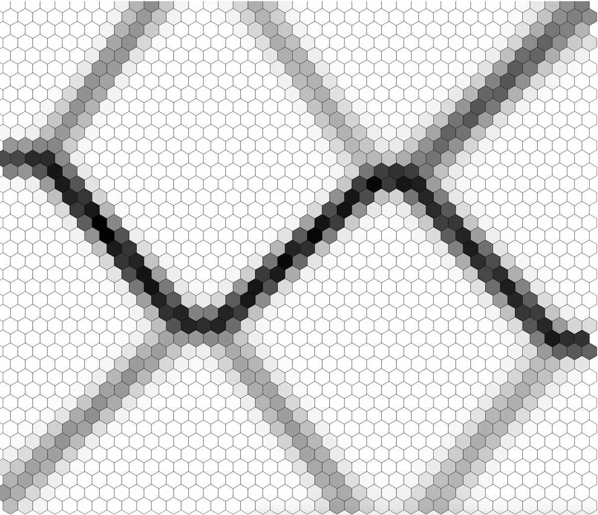
Once the training finishes, we can display the resulting codebook in what’s called U-matrix. UMatrix function generates a simple umatrix image in a specified format. At the moment only SVG format is supported, but feel free to open a PR if you’d like different options :-)
        if err := m.UMatrix(file, d.Data, d.Classes, format, title); err != nil {
                fmt.Fprintf(os.Stderr, "\nERROR: %s\n", err)
                os.Exit(1)
        }
Finally, gosom provides an implementation of a few SOM quality measures that help you calculate quantization error, which measures the quality of the data projection. You can use QuantError function for this. Som topography can be quantified by calculating its topopgraphy error and topography product available via TopoError and TopoProduct functions.
Examples
gosom provides two simples examples available in the project’s repo. The examples both demonstrate the practical uses of the package as well as the correctness of training algorithm implementations. Let’s have a look at one of the examples which is sort of a “schoolbook” example of using SOM for clustering data. Let’s generate a “pseudo-chaotic” RGB image and try to sort it’s colors using SOM. The code to generate the image is pretty simple:
func main() {
        // list of a few colors
        colors := []color.RGBA{
                color.RGBA{255, 0, 0, 255},
                color.RGBA{0, 255, 0, 255},
                color.RGBA{0, 0, 255, 255},
                color.RGBA{255, 0, 255, 255},
                color.RGBA{0, 127, 64, 255},
                color.RGBA{0, 0, 127, 255},
                color.RGBA{255, 255, 51, 255},
                color.RGBA{255, 100, 67, 255},
        }
        // create new 40x40 pixels image
        img := image.NewRGBA(image.Rect(0, 0, 40, 40))
        b := img.Bounds()
        for y := b.Min.Y; y < b.Max.Y; y++ {
                for x := b.Min.X; x < b.Max.X; x++ {
                        // choose a random color from colors
                        c := colors[rand.Intn(len(colors))]
                        img.Set(x, y, c)
                }
        }

        f, err := os.Create("out.png")
        if err != nil {
                log.Fatal(err)
        }
        defer f.Close()

        if err = png.Encode(f, img); err != nil {
                log.Fatal(err)
        }

}
This will generate an image that looks sort of like this:
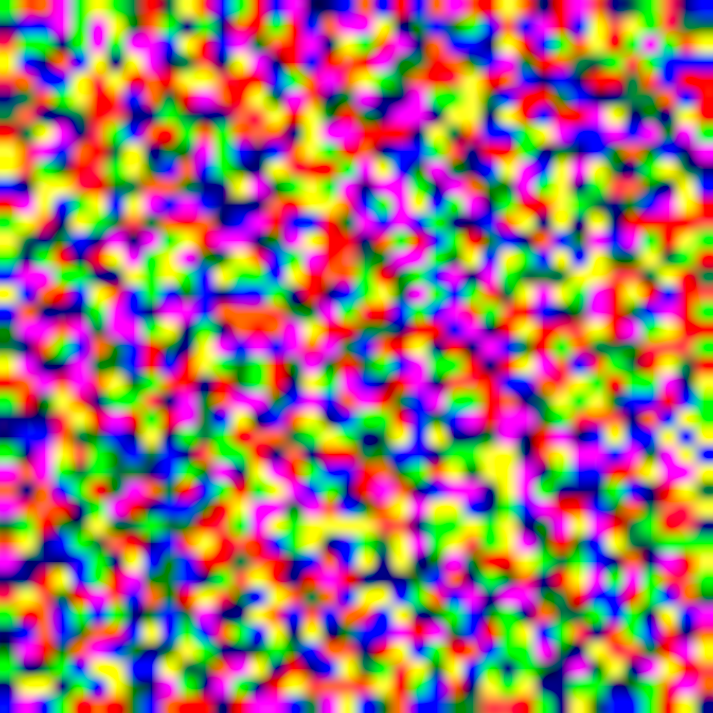
It’s a pretty nice pixel chaos. Let’s use SOM to organize this chaos into clusters of different colors and display it. I’m not going to show the actual code to do this as you can find the full example in the Github repo. SOM training data is encoded into a matrix of 1600x4 . Each row contains R.G.B and A color values. If we now use SOM to cluster the image data and display the resulting codebook on the image we will get something like this:
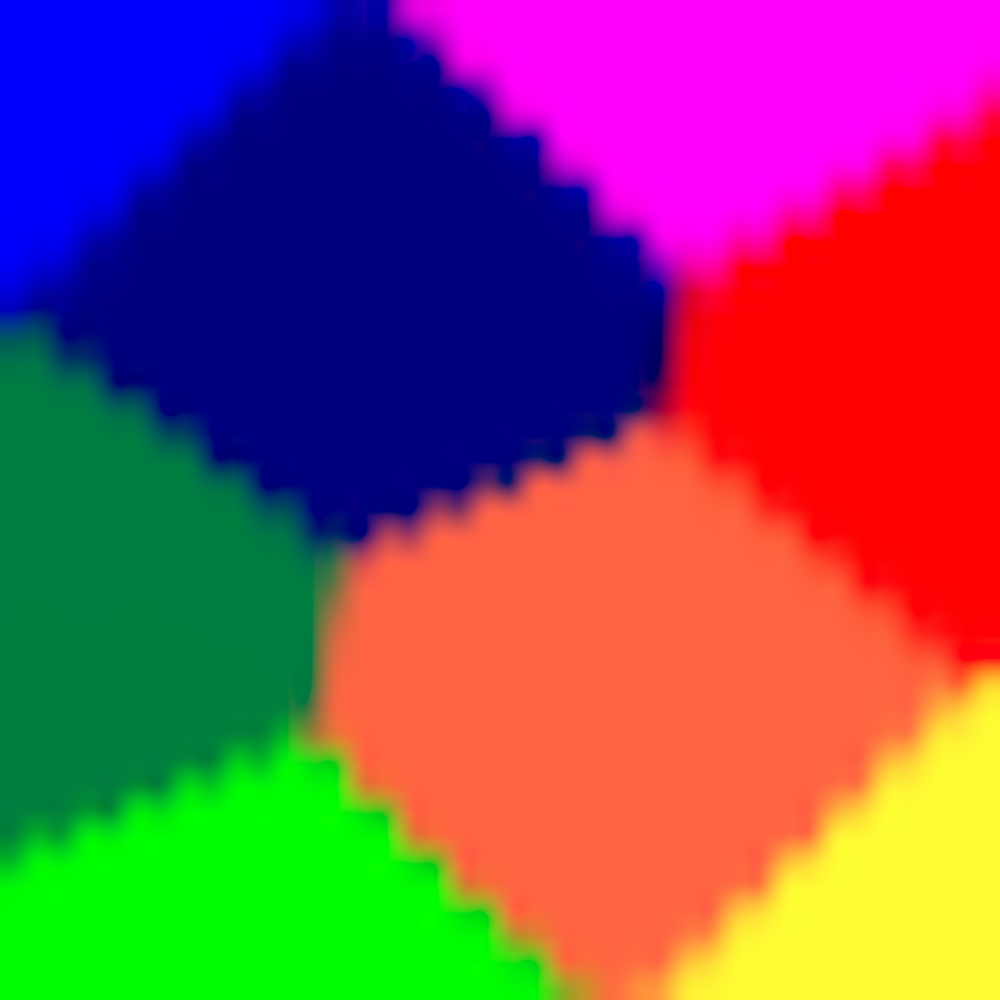
We can see that the SOM created nice pixel clusters of related colors. We can also display u-matrix which looks as below and which basically confirms the clusters visible in the color image shown above:
This concludes our tour of gosom. Feel free to inspect the source code and don’t hesitate to open a PR :-)
Conclusion
Thank you for reading all the way to the end! I hope you enjoyed reading this post at least as much as I enjoyed writing it. Hopefully you have even learnt something.
We talked about Self-organizing maps, a special kind of Artificial Neural Network which is useful for non-linear data projection, feature generation, data clustering, data visualization and in many more tasks.
The post then introduced project gosom, SOM implementation in Go programming language. I explained its basic usage on a simple example and finished by showing its usage on sorting colors in a “chaotic” image.
Self-organizing maps are a pretty powerful type of ANN which can be found in use in many industries. Let me know in the comments if you come up with any interesting use case and don’t hesitate to open a PR or issue on Github.