My rekindled interest in Machine Learning turned my attention to Neural Networks or more precisely Artificial Neural Networks (ANN). I started tinkering with ANN by building simple prototypes in R. However, my basic knowledge of the topic only got me so far. I struggled to understand why certain parameters work better than others. I wanted to understand the inner workings of ANN learning better. So I built a long list of questions and started looking for answers.
“I have no special talents. I am only passionately curious.” – Albert Einstein
This blog post is mostly theoretial and at times quite dense on maths. However, this should not put you off. The theoretical knowledge is often undervalued and ignored these days. I am a big fan of it. If nothing else, understanding the theory helps me avoid getting frustrated with seemingly inexplicable results. There is nothing worse than not being able to reason about the results you program produces. This especially more important in machine learning which is by default an ill-posed maths problem. This post is merely a summary of the notes I made when exploring ANN learning. It’s by no means a comprehensive summary. Nevertheless, I hope you will find it useful and maybe you’ll even learn something new.
If you find any mistakes please don’t hesitate to leave a comment below. I will be more than happy to learn from you and address any inaccuracies in the text. Let’s get started!
Artificial Neural Networks (ANN)
There are various kinds of artificial neural networks. Based on a task particular ANN performs we can roughly divide them into the following groups:
- Regression - ANN outputs (predicts) a number based on input data
- Robotics - ANN uses sensor outputs as inputs and produces some output[s]
- Vision - ANN processes digital images trying to understand them in some way
- Optimization - ANN finds the best set of values to solve some optimization problem
- Classification - ANN classifies data into arbitrary number of predefined groups
- Clustering - ANN clusters data into groups without any apriori knowledge
In this post I will only focus on classification neural networks which are often referred to simply as classifiers. More specifically, I will talk about Feedforward ANN classifiers. Most of the concepts I will discuss in this post are applicable to other kinds of ANN, too. I will assume you have a basic understanding of what a Feedforward ANN is and what components it consists of. I will summarize the most important concepts on the following lines. If you want to dig in more depth, there is plenty of resources available online. You can see an example of a 3-layer feedforward ANN on the image below:
The above feedforward network has three layers: input, hidden and output. Each layer has several neurons: \(4\) in input layer, \(4\) in hidden layer and \(2\) in the output layer. Feedforward neural network is a fully connected network: all the neurons in neighbouring layers are connected to each other. Each neuron has a set of network weights assigned which serve to calculate a weighted input (let’s mark it as z) to the neuron’s activation function. You can see how this works if we zoom in on nne neuron:
From the image above it should be hopefully obvious that network weights allow to control the output of particular neuron (activation) and thus the overall behaviour of the neural network. Input neurons have unit weights (i.e. each weight is equal to \(1\)) and their activation function is [often] what’s referred to as identity function. Identity activation function \(f(x)\) simply “mirrors” the neuron input to its output i.e. \(f(x) = x\). The feedforward network shown on the first image above has two output neurons; it can be used a simple binary classifier. ANN classifiers can have arbitrary number of outputs. Before we dive more into how the ANN classifiers work, let’s talk a little bit about what a classification task actually is.
Note: The above mentioned ANN diagram doesn’t make the presence of neural network bias unit obvious. Bias unit is present in every layer of feedforward neural network. Its starting value is often set to \(1\), although some research documents that initializing the bias input to a random value from uniform Gaussian distribution with \(\mu=0\) (mean) and \(\sigma=1\) (variance) can do just fine if not better. Bias plays an important role in neural networks! In fact, bias units are at the core of one of the most important machine learning algorithms. For now, let’s keep in mind that bias is present in every layer of feedforward neural network and plays an important role in neural networks.
Classification
Classification can be [very] loosely defined as a task which tries to place new observations into one of the predefined classes of objects. This implies an apriori knowledge of object classes i.e. we must know all classes of objects into which we will be classifying newly observed objects. A schoolbook example of a simple classifier is a spam filter. It marks every new incoming email either as a spam or not spam. Spam filter is a binary classifier i.e. it works with two classes of objects: spam or not spam. In general we are not limited to two classes of objects; we can easily design classifiers that can work with arbitrary number of classes.
Note: In practice, most spam filters are implemented using Bayeseian learning i.e. using some advanced Bayesian network or its variation. This does not mean that you can’t implement spam filter using ANN, but I thought I’d point this out.
In order for ANN to classify new data into a particular predefined class of objects we need to train it first. Classifiers are often trained using supervised learning algorithms. Supervised learning algorithms require a labeled data set. Label data set is a data set where each data sample has a particular class “label” assigned to it. In case of spam filter we would have a data set which would contain a large number of emails each of which would be known in advance to be either spam or not spam. Learning algorithm adjusts neuron weights in hidden and output layers so that the new input samples are classified to the correct group. Supervised learning algorithms differ from “regular” computer science algorithms in way that instead of turning inputs into outputs they consume both inputs and outputs and “produce” parameters that allow to fit new inputs into outputs:
Learning algorithm literally teaches the ANN about different kinds of objects so that it can eventually classify newly observed objects automatically without any further help. This is exactly how we as humans learn, too. Someone has to tell us first what something is before we can make any conclusion about something new we observe. If you dive a little bit into neuroscience you will find out that our brain is a very powerful classifier. Classification is a skill we are born with and we often don’t even realize it. Take for example how often do we refer to insect as flies, mosquitos etc. We hardly ever use their real biological names. It’s too costly for our brain to remember the name of every single object in the world. Our brain classifies these objects into existing groups automatically without our too much thinking. Before this happens automatically we are “trained” (taught), so that our brain doesn’t classify flies as something like airplanes.
Backpropagation
Neural network training is a process during which the network “learns” neuron weights from a labeled data set using some learning algorithm. There are two kinds of learning algorithms: supervised and unsupervised. ANN classifiers are often trained using the former, though often the combination of both is often used in practice. This blog post will discuss the most powerful supervised learning algorithms used for training feedforward neural networks: Backpropagation.
Behind every learning (not just ANN learning) is a concept of reward or penalty. Either you are rewarded when you learnt something (measured by answering particular set of questions) or you are penalized if you didn’t (failed to answer the question or answered it incorrectly). Backpropagation, like many other machine learning algorithms, uses the penalty approach. To measure how good the ANN classifier is we define a cost function sometimes referred to as objective function. The closer the output produced by ANN is to the expected value, the lower the value of the cost function for a particular input is i.e. we are penalized less if we produce correct output.
At the core of the backpropagation algorithm is partial derivative of the cost function with respect to its weights and biases i.e. \(\frac{\partial C}{\partial w}\), \( \frac{\partial C}{\partial b} \) where \(C\) is the cost function and \(w\) and \(b\) are network weights and biases. Backpropagation effectively measures how much the cost changes with regards to changing network weights and biases. Neural networks are quite complex and understanding how they work can be challenging. Backpropagation summarises the overall ANN behavior in a few simple equations. In this sense backpropagation provides a very powerful tool to understand ANN behavior.
I’m not going to explain how backpropagation works in this post in too much detail. There is plenty of resources available online if you want to dig more into it. In a gist, backpropagation calculates errors in outputs of neurons in each network layer all the way back from the output layer to the output of the first hidden layer. It then adjusts the weights and biases of the network (this is the actual learning) in a way that minimizes the error in the output layer computed by the cost function \(C\). The error of the output layer is the most important one for the result, but we need to calculate the errors of each particular layer as these errors propagate through the network and thus affect the network output.
I would encourage you to dive more into the underlying theory. There is a real geeky calculus beauty to the algorithm which will give you a very good understanding of one of the most important machine learning algorithms out there. Instead of explaining the algorithm in much detail, I decided to summarize it in two points which I believe are the most crucial for understanding the behavior of feedforward neural network classifiers:
- Cost function is a function of the output layer i.e. it is a function of output neuron activations.
- Learning slows down if any of the “input” neurons is “low-activation”, or if any of the “output” neuron has saturated.
The first point should hopefully be pretty intuitive from the earlier network diagram. We push some input through the network, which produces some output by the output layer neurons. This output is used to calculate the error (cost) with regards to the expected output (label) acccording to the chosen cost function.
Let’s zoom in at the second point: learning slowdown. Learning slowdown, in the context of ANN, means the slowdown of the network weights (and bias) change during the run of the training algorithm. Like I said before, backpropagation changes the network weights with regards to the calculated error for given input and expected output. Change of the weights is the core of the learning. When the weights stop changing during backpropagation, the learning stops as the cost no longer changes, hence we can improve the output of the network. By doing a little bit of calculus we could show that backpropagation learning depends on derivation of the activation function. We could sum this up using a simple equation below:
$$ \frac{\partial C}{\partial w} = a_{in}.\delta_{out} $$
where \(C\) is the cost function, \(a_{in}\) is the activation (i.e. the output produced by the neuron) of neuron that is an input to network weight \(w\) of another neuron in the next layer and \(\delta_{out}\) is the error of the neuron output from the weight \(w\). The picture below should give you a better idea about the equation above:
We could further show that the error \(\delta_{out}\) depends on a derivation of the activaion of the intermediary neuron in the output produced by neuron with weights \(w\) (remember derivation is always defined in some point - in our case that point is output produced by a particular neuron). The most important implication of this equation for network learning is that the change of cost with regards to change of weights depends on the activation input into weight \(w\), \(a_{in}\), and on activation function derivation in the point equal to output of the neuron with weights \(w\). Clearly, activation function plays a crucial role in how fast the neural networks can learn, so it’s a topic worth exploring further.
One of the most well known activation functions is sigmoid function often referred to simply as sgmoid. Sigmoid is well known to be used in logistic regression. Sigmoid holds some very interesting properties which make it a natural choice of neuron activation function in ANN classifiers. If we look closely on the sigmoid function on the graph below we can see that it resembles a continuous approximation of step function found in transistor switches which can be used to signal binary output (on or off). In fact, we could show that by tuning sigmoid parameters we could get a pretty good approximation of the step fuction. The ability to simulate a simple switch with boolean behavior is handy for classifiers which need to decide whether the newly observed data belongs to a particular class of objects or not.
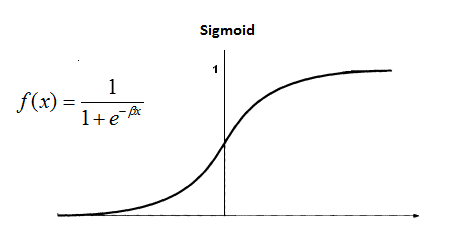
I mentioned earlier that if the output neuron saturates then the network stops learning. Saturation means there is no rate change happening which means the derivative in any saturation point is \(\approx 0\). This means that the partial derivation of cost function by weights in the equation mentioned earlier tends to get to \(\approx 0\). This is exactly the case with sigmoid function. Notice on the graph above how sigmoid eventually saturates on \(0\) (when \(x \ll 0\)) or \(1\) (when \(x \gg 0\)). Sigmoid suddenly doesn’t seem like the best choice for the activation function, at least not for the network output neurons. Luckily, by choosing a particular kind of cost function we can subdue the effect of neuron saturation to some degree. Let’s have a look at what would such cost function look like.
Cost function and neuron activations
Cost function is a crucial concept for many machine learning algorithms, not just backpropagation. It measures the error of computed output for a given input with regards to expected result. Cost function output must be non-negative by definition. As I will show you later on, good choice of the cost function can hugely improve the performance of ANN learning whilst a bad choice can lead to suboptimal results. There are several kinds of cost functions available. Probably the most well known one is quadratic cost function.
Quadratic cost function calculates mean squared error (MSE) for a given input and expected output:
$$ C = \frac{1}{2n}\sum_{k=1}^{n} \lVert y - a^L \rVert^2 $$
where \(n\) is the number of training samples, \(y\) is the desired output, \(L\) represents the number of layers in ANN, so $$a^L$$ is the activation of the output layer neuron for a particular input.
Whilst MSE is suitable for many tasks in machine learning, we could prove that it’s not the best choice of the cost function for ANN classifiers. At least not for the ones that use the sigmoid activation in the output layer. The main reason for that is that this combination of activation and cost can slow down ANN learning.
We could, however, show by performing a bit of calculus that if the output neurons are linear i.e. their activation function is defined as $$y = x$$, then the quadratic cost function will not cause learning slowdown and thus it can be an appropriate choice of cost function. So why don’t we ditch the sigmoid and go ahead with the linear activations and quadratic cost function combination instead? It turns out linear activations can still be pretty slow in comparison to other activation functions we will discuss later on.
So what should we do if our output layer neurons use sigmoid activation function? We need to find a better cost function than the quadratic cost, which will not slow down the learning! Luckily, there is one we can use instead. It’s called cross-entropy function.
Cross-entropy cost function
Cross-entropy is one of the most widely used cost functions in ANN classifiers. It is defined as follows:
$$ C = -\frac{1}{n}\sum_{k=1}^{n} y^{(k)}log(a^{(k)}) + (1-y^{(k)})log(1-a^{(k)}) $$
where \(n\) is the total number of training samples, \(y^{(k)}\) is expected output for a particular input and \(a^{(k)}\) is an output activation for the given input.
It’s important to point out that if you do decide to use the cross entropy cost function you must design your neural network in the way that contains as many outputs as there are classes of objects. Additionally the expected outputs should be mapped into one-of-N matrix. Having this in mind, you can start seeing some sense in the cross entropy function. Befor I explain in more defatil that cross-entropy cost addresses the problem of learning slowdown when using the sigmoid activation, I want to highlight some important properties it holds:
- it’s a non-negative function (mandatory requirement for any cost function)
- it’s a convex function (this helps to prevent getting stuck in local minimum during learning)
Notice that if \(y^{k} = 0\) for some input then the first term in the above equation sum addition disappears. Equally if \(y^{k} = 1\) the same thing happens with the second term. We can therefore break down the cross-entropy cost function into following definition:
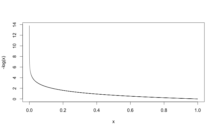
$$ C = \begin{cases} -log(a) &\text{if } y = 1 \\ -log(1-a) &\text{if } y = 0 \end{cases} $$
where \(y\) is expected output and \(a\) is neural network output. Plotting the graphs for both cases should give us even better understanding.
In the first case we are expecting the output of our network to be \(y = 1\). The further the ANN output is from the expected value (\(1\)), the higher the error and the higher the cost output:
In the second case, we are expecting the output of our network to be \(y = 0\). The closer the output of our network is to the expected output (\(0\)), the smaller the cost and vice versa:
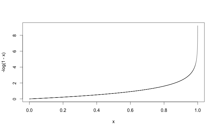
Based on the graphs above we can see that cross-entropy tends to converge towards zero the more accurate the output of our network gets. This is exactly what we would expect from any cost function.
Let’s get back to the issue of learning slowdown. We know that at the heart of the backpropagation algorithm is a partial derivative of cost function by weights and biases. With a bit of calculus we can prove that when using cross-entropy as our cost function and sigmoid for activation in the output layer, the resulting partial derivative does not depend on the rate of change of activation function. It merely depends on the output produced by it. By choosing the cross-entropy we can avoid the learning slowdown caused by the saturation of the sigmoid activation function.
If your output neurons use sigmoid activation it’s almost always better to use corss-entropy cost function.
Hyperbolic tangent activation function (tanh)
Before we move on to the next parargraph, let’s talk shortly about another activation function whose properties are similar to the sigmoid function: hyperbolic tangent, often referred to simply as tanh. Tanh is in fact just a rescaled version of sigmoid. We can easily see that on the plot below:
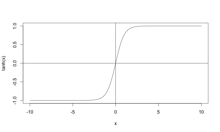
Similar to the sigmoid, tanh also saturates, but in different values: \(-1\) and \(1\). This means you might have to “normalize” the output of the tanh neurons. Once your tanh outputs are normalized you can use the cross-entropy cost function in backpropagation algorithm. Some empirical evidence suggests that using tanh instead of sigmoid provides better results for some learning tasks. However, there is no rigorous proof that tanh outperforms sigmoid neurons, so my advice to you would be to test both and see which one performs better for your particular classification task.
Softmax activation and log-likelihood cost function
By using cross-entropy function in combination with sigmoid activation we got rid of the problem with saturation, but the learning still depends on the output of the activation function itself. The smaller the output the slower the learning gets. We can do better as we will see later on, but first I would like to talk a little bit about another activation function which has found a lot of use in ANN classifiers and in deep neural networks: softmax function, often referred to simply as softmax. Softmax has some interesting properties that make it an appealing choice of the output layer neurons in ANN classifiers. Softmax is defined as below:
$$ a_i = \frac{e^{z_i}}{\sum_{k=1}^{n} e^{z_k}} $$
where \(a_i\) is activation of \(i\)-th neuron and \(z_i\) is input into activation of \(i\)-th neuron. The denominator in the softmax equation simply sums “numerators” across all neurons in the layer.
It might not be entirely obvious why and when should we use softmax instead of sigmoid or linear activation functions. As always, the devil lies in the details. If we look closely at the softmax definition, we can see that each activation \(a_i\) represents its proportion with regards to all activations in the same layer. This has an interesting consequence for the other neuron activations. If one of the activations increases the other ones decrease and vice versa i.e. if one of the neurons is dominant, it “subdues” the other neuron outputs. In other words: any particular output activation depends on all the other neuron activations when using the softmax function i.e. particular neuron output no longer depends just on its weights like it was the case with sigmoid or linear activations.
Softmax activations of all neurons are positive numbers since the exponential function is always positive. Furthermore, if we sum softmax activations across all neurons in the same layer, we will see that they add up to \(1\):
$$ \sum_{i=1}^{n} a_i = 1 $$
Given the above described properties we can think of the output of softmax (by output we mean an array of all softmax activation in particular network layer) as a probability distribution. This is an excellent property to have in ANN classifiers. It’s very convenient to think of an output neuron activations as a probability that particular output belongs to a particular class of objects. For example we can think of \(a_i\) in the output layer as an estimate of the probability that the output belongs to the \(i\)-th object class. We could not make such assumption using sigmoid function as it can be proved that the sum of all activations of sigmoid function in the same layer does not always add up to \(1\).
We have shown earlier that by clever choice of cost function (cross-entropy) we can avoid learning slowdown in ANN classifiers when using sigmoid activations. We can pull the same trick with softmax function. Again, it will require a different cost function than the cross-entropy. We call this function log-likelihood. Log-likelihood is defined as below:
$$C = -log(a^{L}_{y_{k}})$$
where \(L\) is the last network layer and \(y_{k}\) denotes that the expected output is defined by class \(k\).
Just like cross-entropy, log-likelihood requires us to encode our outputs into on-of-N matrix. Let’s have a closer look at this cost function like we did with cross-entropy. The fact that the output of softmax can be thought of as a probability distribution tells us two things about the cost function:
- The closer the particular output is to the expected value is, the closer its output is to \(1\) and the closer the cost tends to get to \(0\).
- The further the particular output is from the expected value, the closer its output is to \(0\) and the cost tends to grow to infinity.
The log-likelihood behaves exactly like we would expect the cost function to behave. This can be seen on the plot below:
So how does softmax address learning slowdown? By performing a bit of calculus we could once again show that partial derivative of log-likelihood by weights (\(\frac{\partial C}{\partial w}\)), which is a at the core of backpropagation algorithm, merely depends on the output produced by activation output just like it was the case with sigmoid and cross-entropy. In fact, softmax activation and log-likelihood perform quite similar as sigmoid and cross-entropy. So when should you use which one? The answer is it depends. A lot of influential research in ANN space tends to use softmax and log-likelihood combo which has a nice property if you want to interpret the output activations as probabilities of belonging to a particular class of objects.
Rectifier linear unit (ReLU)
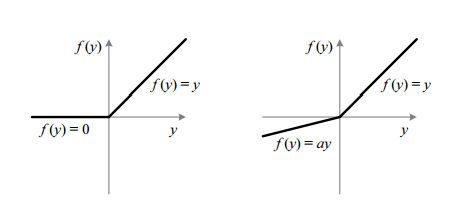
Before we move on from the topic of activation functions, I must mention one last option we have at our disposal: rectifier linear unit, often referred to simply as ReLU. ReLU function is defined as follows:
$$ f(x) = \begin{cases} x &\text{if } x > 0 \\ 0 &\text{if } x \le 0 \end{cases} $$
ReLU has been an active subject of interest of ANN research. Over the years it has become a very popular choice of activation function in deep neural networks used for image recognition. ReLU is quite different from all the previously discussed activation functions. As you might have noticed on the plot above, ReLU does not suffer from saturation like tanh or sigmoid functions as long as its input is greater than \(0\). When the ReLU input is negative, the ReLU neurons stop learning completely. To address this, we can use a similar function which is a variation of ReLU: Leaky ReLU (LReLU).
LReLU is defined as follows:
$$ f(x) = \begin{cases} x &\text{if } x > 0 \\ 0 &\text{if } ax \le 0 \end{cases} $$
where \(a\) is a small constant which “controls” a slope of LReLU output for the case of negative values. The actual value of the constant can differ for different use cases. The best I can advise you is to experiment with different values and pick the one that gives you the best results. LReLU provides some improvement in learning in comparison to the basic ReLU, however the improvement can be negligible. Worry not, there seems to be a better alternative.
You can find plots of both ReLU and LReLU on the picture below:
A group of Microsoft researchers achieved some outstanding results in image recognition tasks using another variation of ReLU called Parametric Rectifier Linear Unit (PReLU). You can read more about the PReLU in the following paper. You will find out, PReLU is just a “smarter” version of LReLU. Whilst LReLU forces you to choose the slope constant \(c\) before you kick off the learning, PReLU can learn the slope constant \(c\) during backpropagation. Furthermore, whilst LReLU slope constant is static i.e. it stays the same for all neurons during the whole training, PReLU can have different slope values for different neurons at different states of the training!
The question now is, which one of the ReLU activations should we use? Unfortunately there does not seem to exist any rigorous proof or theory about how to choose the best type of rectifier linear units and for which tasks it is the most suitable choice of neuron activation. The current state of knowledge is based heavily on empirical results that show that rectifier units can improve the performance of restricted boltzman machines, acoustic models and many other tasks. You can read more about evaluation of different types of rectifier activation function used in convolutional networks in the following paper.
Weights initialization
Choosing the right neuron activations with appropriate cost function can clearly influence the performance of ANN. But we can go even further. I found out during my research the network weights initialization can play an important role in the speed of learning. This was a bit of a revelation to me. I would normally go ahead and initialize all neuron weights in all hidden layers to values from Gaussian distribution with \(0\) mean and standard deviation \(1\) without too much thinking. It turns out there is a better way to initialize the weights which can increase the speed of learning!
So what is wrong with choosing \(\mu=0\) and \(\sigma=1\) parameters of Gaussian distribution I mentioned earlier? Imagine a situation when a significant number of neuron inputs are \(\approx 0\). This is not an unusual situation. As you could see earlier, sigmoid or ReLU can easily produce values \(\approx 0\) if the neurons inputs are \(\ll 0\). When that’s the case, the weighted output of the neurons (i.e. the input into the neuron activation function) in the next layer can produce values of Gaussian distribution whose standard deviation is \(\gg 0\) (the actual value depends on number of neurons). The problem with large standard deviation of activation input is that it causes the saturation of the neuron outputs. As we learnt earlier this has a consequence of learning slowdown.
We can avoid this problem by choosing a better set of Gaussian distribution parameters for weight initialization. There is no exact formula what should the standard deviation of weight initialzation be, but some research suggests that by choosing the standard deviation to be around the inverse of the square root of number of input weights (\(\approx \sqrt{1/n}\)) should give you better performance than the uniformly distributed values I mentioned at the beginning of this discussion. If we plot the values of both network weights distributions for both cases it could look something like the plot below:
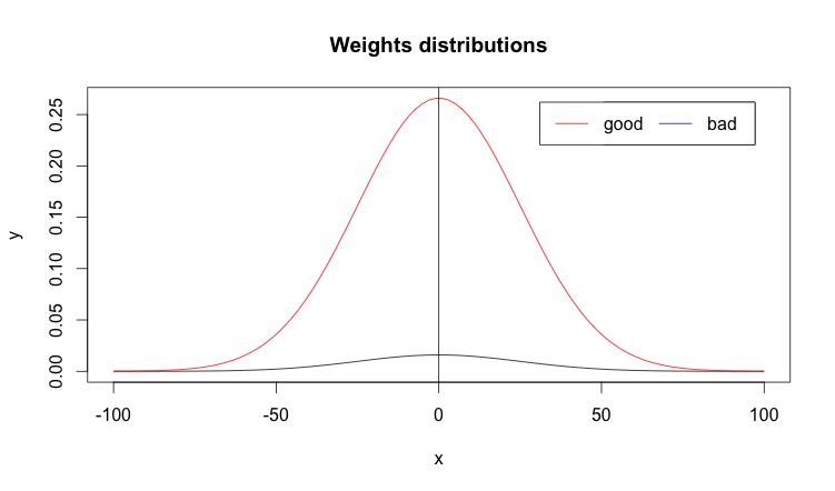
You should spot straight away that the distribution we are aiming for is much sharper i.e. its bell curve is much steeper. Low standard distribution helps to avoid neuron saturation and speeds up ANN learning, which is what we are striving for. You may have noticed that I did not mention how to initialize weights of bias neurons. It turns out, the weights initialization of bias neuron does not play any significant role in ANN learning so it should be ok to stick to the original standard deviation \(1\) without worrying too much.
Learning optimization
The goal of ANN learning algorithm is to find network weights for which the output of the cost function is as minimal as possible. This is clearly an optimization problem: we need to find weights that niminimize the output of the cost function. One of the most famous optimization algorithm used to solve this problem is called gradient descent. I’m not going to discuss the gradient descent algorithm here. Again, there is plenty of resources online if you want to understand it. And I would strongly advise you to do so, as gradient descent has huge number of applications, not only in machine learning.
Instead, I would like to mention some alternative solutions. In particular, I would like to talk shortly about some advanced optimization algorithms you can use instead of gradient descent. There are several options available at our disposal. Probably the most well known is Broyden–Fletcher–Goldfarb–Shanno, often referred to simply as BFGS and its limited memory alternative L-BFGS. Another alternative would be Conjugate gradient.
Why do I mention these advanced optimization methods? First of all, majority people are well aware of the gradient descent and so was I when I started doing my research. At some point I came across Yann LeCun’s paper on efficient backpropagation which discusses them in broader detail. These algorithms can seem very complicated, but their efficient implementations are available in many numerical toolboxes. Their biggest advantage is they don’t require much tuning. At least not as much as gradient descent. There is no need to pick many parameters except for number of iterations we want to run them for. They just work and if implemented properly they often outperform gradient descent. They are often more suitable choice for large machine learning problems which deal with huge data sets than gradient descent. If these algorithms are so good why do so many people still rely on good old gradient descent or any of its variations?
The answer, as it often is in the world of science (or life in general), is the complexity. Like I already mentioned, some of these algorithms are quite advanced and not easy to understand for some people. This can make their debugging quite hard. Often their implementations differ between various toolboxes which makes their debugging even harder. Finally, gradient descent performance is often acceptable and much better understood. It’s good to be aware that these algorithms exist and are available to use.
Neural networks in Go
Armed with the newly gained knowledge I could finally have a better understanding of neural networks. But I didn’t want to stay in theory. After all a certain wise man once said something which I find incredibly true:
“What I can not create I do not understand” – Richard Feynman
I’ve been a big fan of Go language for a while and I wondered on and off how well does it perform in numerical computations. After doing a bit of research I found the awesome gonum project that contains a great wealth of numerical packages. I took them for a spin and to my great joy, I found out that the gonum packages are pretty damn fast as long as you take advantage of the vectorised operations. Gonum is one of the biggest gems in the Go ecosystem, so do not hesitate and spend some time exploring the packages in it - you won’t regret!
The result of my hacks is a small project. I am well aware of the awesome projects like go-ml or golearn and many many others. The main reason why I decided create my own implementation despite many a people discouraging me as it being a waste of time was for purely learning experience and therefore the project itself should therefore be treated accordingly :-) You might find it useful and maybe it will even inspire you to hack on your own, improved implementation. The learning experience I got from this was priceless!
Conclusion
We have finally reached the end of the post. Thank you very much for reading! It’s been a long ride! We learnt about various techniques that can help us speed up ANN learning. We learnt about learning slowdown and how we can address it by choosing appropriate combination of neuron activations and cost function. Based on the research I’ve done, it seems the most popular choice of neuron activation function in classification tasks is some varioation of ReLU for the hidden layer neurons (to model system’s non-linearities) and softmax activation for the output layer neurons. The presence of softmax in the output layer “dictates” the use of log-likelihood cost function. As always, YMMV and the particular choice might differ based on the taks your network performs. All you need to do is to roll up your sleeves and make some experiments.
Writing this blog post has been amazing personal journey for me. It made me revisit some old knowledge of neural networks theory and learn tonnes of new stuff from many research papers I had not heard of before. I hope you have enjoyed reading thist post as much as I have writing it. If you have any comments, do not hesitate to leave them below.