This is the second post of the series about Principal Component Analysis (PCA). Whilst the first post provided a theoretical background, this post will discuss the actual implementation of the PCA algorithm and its results when applied to some example data.
Theory Recap
In the first post we learnt that PCA looks for a vector basis that can express the analysed data in a better (less redundant) way, whilst retaining as much information from the original data as possible. The vectors that form this vector basis are called principal components.
We learnt that the princpal components point the direction of highest variance. The hope behind this thinking is that the variance along a small number of principal components (i.e. less than the number of measurement types) provides a reasonably simplified model of the complete data set.
Finally, we learnt that PCA assumes that the principal components are orthogonal which makes finding them a problem solvable using linear algebra.
Eigenvectors and diagonal matrix
The previous post introduced a concept of covariance matrix as an important construct that can help to reveal signal and noise in our data. The solution to finding principal components takes advantage of some of the properties covariance matrix exhibits.
We know that covariance matrix is a square symmetric matrix. We also know that in ideal case the covariance matrix should be a diagonal matrix with variances on its diagonal and all the off-the diagonal values equal to zero. The solution to PCA lies in finding a way that diagonalizes the covariance matrix.
From linear algebra we know that for a symmetric matrix \(S\), we can find a matrix \(E\) such that the following equation holds true:
$$ S = EDE^T $$
where matrix \(D\) is a diagonal matrix and \(E\) is a matrix that contains eigenvectors of matrix \(S\) stored in its columns. Eigenvectors always come in pairs with eigenvalues. Whilst the eigenvectors of covariance matrix carry the information about the direction of the highest variance, eigenvalues provide a measure of its proportion. Put another way: the higher the eigenvalue of the eigenvector the more information can be found in its direction.
Let’s go back to the original matrix equation PCA tries to solve:
$$XB= X’$$
where \(X\) is the data matrix we are trying to express using the vector basis stored in the columns of matrix \(B\). The result of the transformation is a new matrix \(X’\).
Let’s create a covariance matrix \(C_{X’}\) from matrix \(X’\) i.e. the covariance matrix of the transformed data set. Let’s assume that each column of \(X’\) is mean-centered so we can express \(C_{X’}\) as follows:
$$ C_{X’} = \frac{1}{n}X’^TX’ $$
We can rewrite this equation using \(X\) like this:
$$ C_{X’} = \frac{1}{n}(XB)^T(XB) = B^T(\frac{1}{n}X^TX)B $$
We can see that the covariance matrix of the transformed data can be expressed using the covariance matrix of the original data matrix:
$$ C_{X’} = B^TC_XB $$
We also know that \(C_{X}\) is a symmetric matrix, so the previous formula can be be express like this:
$$ C_{X’} = B^TC_XB = B^T(EDE^T)B $$
If we now choose the matrix \(B\) so that it contains eigenvectors of covariance matrix \(C_{X}\) in its columns, i.e. \(B = E\), we can show that \(C_{X’}\) is diagonal:
$$ C_{X’} = D $$
This result takes advantage of an important property of eigenvectors: \(E^T = E^{-1}\). Since we chose \(B\) so that \(B = E\) we can prove the correctness of the previous equation as follows:
$$ C_{X’} = B^T(EDE^T)B = E^TEDE^TE = (E^{-1}E)D(E^{-1}E) = D $$
We can see that the principal components can be found by finding the eigenvectors of the covariance matrix of the measured data. This finally concludes our quest for finding the principal components.
Algorithm
Armed with this knowledge we can finally formalize the PCA algorithm in a simple step by step summary:
- Construct the data matrix; each row contains separate measurement
- Mean center each column of data matrix
- Calculate the covariance matrix from the data matrix
- Calculate the eigenvectors and eigenvalues of the covariance matrix
- Sort the eigenvectors by the largest eigenvalue
- Profit :-)
Before we go ahead and apply this algorithm on some example data sets, we will shortly discuss some alternative solutions.
Singular Value Decomposition (SVD)
Singular value decomposition is a matrix diagonalization algorithm. It allows to express a matrix in the following form:
$$ X = U \Sigma V$$
where \(\Sigma\) is a diagonal matrix with non-negative numbers on its diagonals and columns of matrices \(U\) and \(V\) are orthogonal. We call the vectors in \(U\) and \(V\) left and right singular vectors respectively. Principal components are the right singular vectors.
We are not going to be discussing SVD in more detail in this post. Just remember that you can use SVD to find the principal components, too. In fact the PCA and SVD are so closely related that the two are almost interchangeable. We will demonstrate this on a practical example later in this post.
Mean square error minimization
Another framework derives the PCA by using its property of minimizing the mean squared error. This is often framed as a projection error problem. In this case, we define a loss (error) function:
$$ J(x) = \frac{1}{n}\sum_{k=1}^{n} \lVert x_k - x’_k \rVert^2 $$
where \(x_k\) are the data measurements, and \(x’_k\) are defined as follows:
$$ x’_k = \sum_{i=1}^{q} (e_i^Tx_k)e_i $$
where vectors \(e_i\) are the orthonormal basis we are trying to find in a way that minimizes the distance between the original data and their projections into the new vector space. Put another way: we are trying find some orthonormal basis \(e_i\) that minimizes the loss function \(J(x)\).
THere is an interesting research happening in this field. Turns out you can do projection without actual PCA.
Examples
It’s time to take the PCA algorithm for a spin and apply it on some data. We will start with the data set described in the first post. You can download it from my repo on GitHub here. The repo also contains the PCA implementation source code in R.
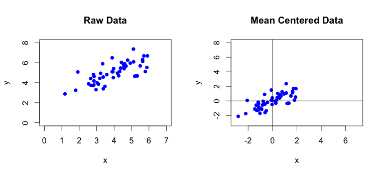
First thing we need to do is to mean center the raw data. Sometimes you will also have to perform feature scaling on the collected data. This is often required when the values of measured features vary by large degree such as when your matrix contains measurements in different units like kilometers and milimeters. By performing feature scaling you make sure that each data feature contributes to the result by approximately the same proportion. Our test data does not require the feature scaling.
You can see the comparison of raw and mean centered data at the following plot:
In the next step we will calculate the covariance matrix from the mean centered data:
$$ C_X = \left[\begin{array} {rrr} 1.3760 & 0.8830 \\ 0.8830 & 1.0474 \end{array}\right] $$
We can notice that the off-the diagonal items are non-zero, which means that the two features in our data are correlated. This means that we should be able to reduce the dimension of this data set!
We now need to calculate the eigenvectors and eigenvalues of the covariance matrix. If you use the R language to calculate these, you can use a handy function called eigen(). This function automatically orders the eigenvectors based on the size of their eigenvalues. You should get the following results:
$$ eigenvalues = \left[\begin{array} {rrr} 2.1098782 & 0.3135314 \end{array}\right] \\ \\ \mathbf{eigenvectors} = \left[\begin{array} {rrr} -0.7690815 & 0.6391507 \\ -0.6391507 & -0.7690815 \end{array}\right] $$
To illustrate that the eigenvectors of the covariance matrix really do highlight the directions of highest variance we will overlay our mean centered data with regression lines defined by the both found eigenvectors:
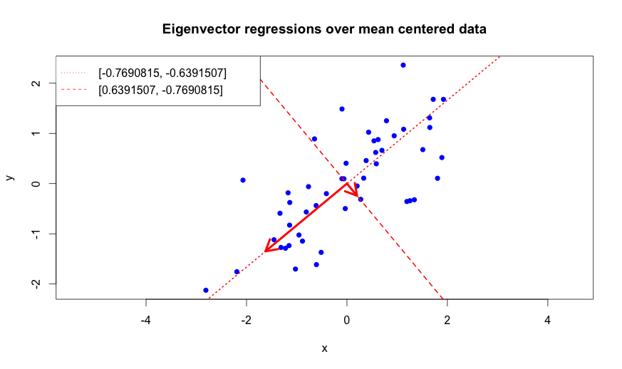
The above rendered plot shows that the eigenvectors are orthogonal to each other like we expected. More importantly, we can see that the line which is defined by the eigenvector with the bigger eigenvalue shows a strong pattern in the data: it approximates the direction of runner’s movement. The second eigenvector “carries” less information. It basically tells us that some data points fluctuate around the line that is parameterized by the first eigenvector.
We will now try to find the principal components using SVD and compare the results to our eigenvector driven algorithm. We know that the principal components are equal to the right singular vectors. When we calculate the SVD of our covariance matrix and look at the matrix \(V\) which contains the right singular vectors we should see the following result:
$$ V = \left[\begin{array} {rrr} -0.7690815 & -0.6391507 \\ -0.6391507 & 0.7690815 \end{array}\right] $$
The column vectors of \(V\) are [almost] exactly the same as the eigenvectors of the covariance matrix we found earlier. The only difference is the sign of the second right singular vector. This does not matter as long as the calculated vectors are orthogonal to each other. Flipping the sign of the vector merely flips its direction to the exact opposite side and has no effect on the variance. This should be obvious from the plot we drew earlier.
Principal components are the vector basis that allows to express the original data in a better way than they were collected. Let’s illustrate this by plotting the data expressed using the new vector basis. We will use our well know matrix transformation equation:
$$ XB = X’$$
Let’s show the comparison between the original and transformed data by drawing a simple plot:
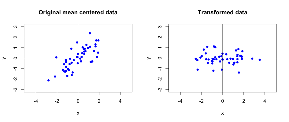
We can see that expressing the original data using the principal components rotated it in a way that describes it better. Principal components transformed the data captured on a camera from some arbitrary angle so that it now highlights the runner’s trajectory. It should be clear that the important information lies along \(x\) axis and the \(y\) values captured by camera are rather redundant and can be removed without losing too much information.
Dimensionality reduction
Dimensionality reduction using PCA is a straightforward task once we know how much information are we willing to lose. This obviously depends on many factors, but in our example we can only reduce the dimension by a single degree. We can measure the information loss by calculating the proportion of lost variance. There are two ways to go about it:
- measure the mean square transformation (projection) error
- measure the proportion of variance captured by particular eigenvalue
In the first case we would calculate the projection error using the following formula:
$$ Error = \frac{\frac{1}{m}\sum_{i=1}^{m} \lVert x^{(i)} - x_{proj}^{(i)} \rVert^2}{\frac{1}{m}\sum_{i=1}^{m}\lVert x^{(i)} \rVert^2} $$
where \(x\) is our mean centerd data and \(x_{proj}\) is the projected data. The upper index \((i)\) is a number of dimensions we decided to keep.
The second case can be formalized using following equation:
$$ VAR_{cap} = \frac{\sum_{i=1}^{m}(eig_i^2)}{\sum_{k=1}^{n}(eig_k^2)} $$
where \(VAR_{cap}\) is a proportion of variance captured by particular eigenvalues \(eig_i\). In our example we would find out that the first principal component (the one with the highest eigenvalue) captures 97.84% of variance. We will accept the ~2% information loss and go ahead and reduce the data dimension in our example. We will use the same transformation equation, but instead of using both principal components we will only use the first one. The result will be a one dimensional matrix i.e. a single column vector.
So now that we know how to transform the data and how to measure the data loss, it’s time to learn how to reconstruct the original data back. Thi is actually pretty simple. All we need to do is to solve our familiar matrix equation:
$$ X = X’ B^{-1} = X’B^T$$
We know that \(X\) contains mean centered data so if we wanted to reconstruct the raw data we would need to add the original mean values of particular features to the result of this equation. We will not peform the full reconstruction from the transformed data. Instead, we will look at reconstrucing the data from the reduced data set. Once we do this, we can plot the results for comparison:
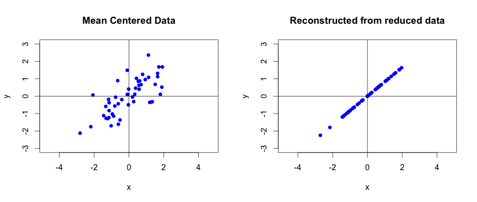
The above plot nicely illustrates the loss of one dimension. Whilst the variance along the eigenvector with the highest eigenvalue has been kept, the data along the second eigenvector has completely disappeared! As we learnt, reducing the data dimension naturally causes data loss. Luckily, according to our previous calculation, this loss is only about 2%. In reality, you would strive for much smaller data loss.
Digital image compression
Before we conclude this post we will have a quick look at one more example which involves digital image processing. We will run the PCA algorithm on some arbitrary image downloaded from the internet:
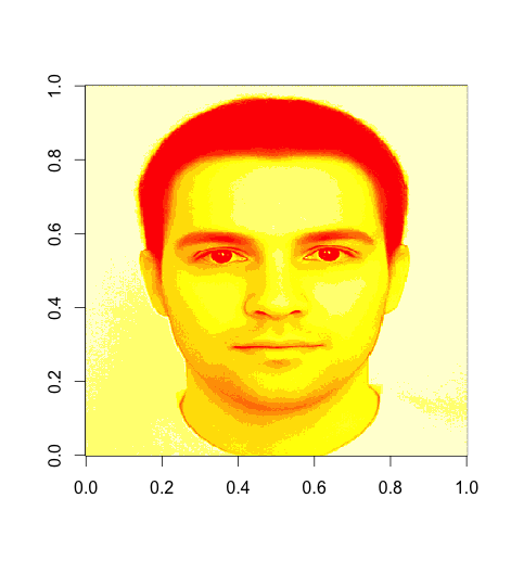
The size of the image is \(400 \times 320\) pixels. For simplicity, we have only used one of the three RGB dimensions. We will now try to find the principal components and perform the dimensionality reduction.
Once we found the principal components we can plot the relatinship between retained proportion of variance and number of principal components:
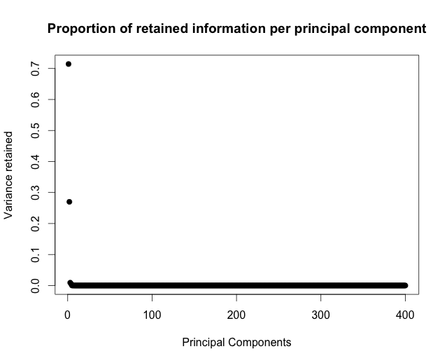
We can see that that the image data can be reasonably well explained by just a few principal components, maybe 6 or 7. These capture over 95% of data variance, which should be good enough for machine processing. Let’s display the compressed image, using the data captured by top 7 principal components:
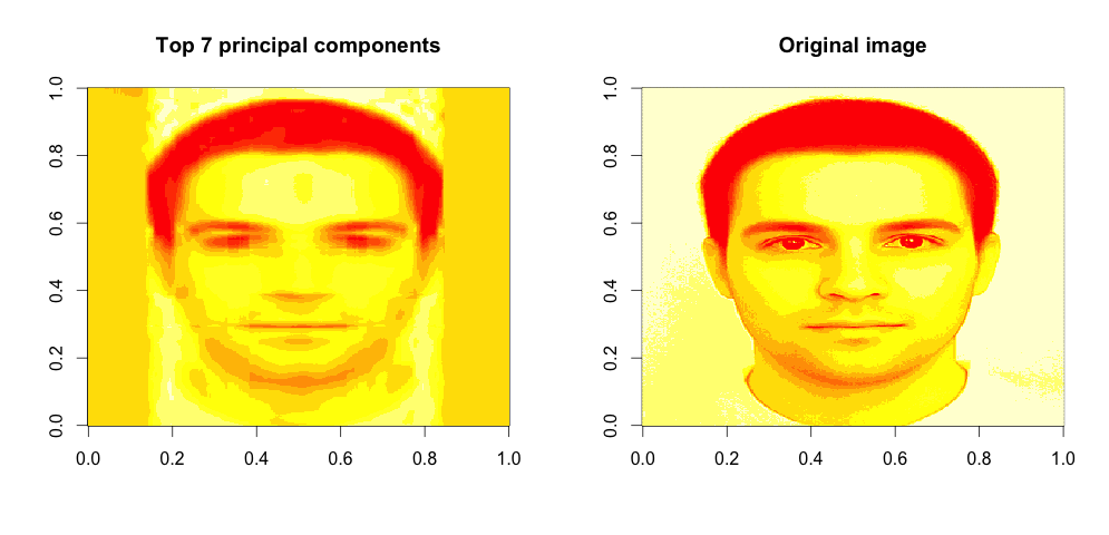
We can identify the person in the picture. This is pretty good, given that we only used \(400 \times 7\) data measurements. which gives us 97.8% data compression of the original data! This means significant processing time gain!
Whilst this result can be good enough for machines, it is not great for the presentation purposes or for any practical tasks done by humans. We can’t properly see all the face features. If we want better precision we need to increase the number of principal components used for compression. We can experiment with different compression levels and compare the results in the graph below:
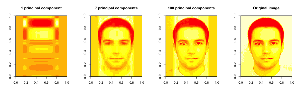
We can see that even the single top principal component does identify the main patterns in image, however the projection is very poor. Using 7 vectors, as we mentioned earlier, gets pretty close, but not great. The higher the number of principal components we use the higher the data variance and better the resulting picture.
Conclusion
In this post we formalized the PCA algorithm in a step by step guide. We have then looked at some practical examples that. First we removed the redundant dimension from the runner’s data and illustrated the importance of eigenvectors. Then we looked at how can we reconstruct the original data from the transformed data set. Finally, we showed how PCA can be used for simple image compression.
I would like to thank you for spending your free time reading this post. gIt was a good fun and learning experience writing it. I hope you enjoyed it and if you spotted any inaccuracies, feel free to leave a comment below.
You can find all the source code in my GitHub repo