This is the first of the two post series about Principal Component Analysis (PCA). This post lays down important knowledge bricks that are needed to understand the core principles of the PCA algorithm. The second post will discuss the actual implementation and its results by applying it to various data sets.
Motivation
The world is becoming more data driven than ever before. We collect large amounts of data from arbitrary sources. This is often because we don’t know which data best describes the systems we are trying to understand. The fear of missing out on capturing important features forces us to collect a lot of redundant data.
Amassing large amounts of data introduces a whole new set of problems. For starters, the more data we collect, the longer it takes to process it. We also find it hard to understand big data sets as we naturally try to visualize them. Visualizing is impossible when the collected data goes beyond three dimensions. Luckily, there has been a lot of research done over the years focused on a lot of big data issues. Principal Component Analysis is one of many algorithms which can help us when making sense of big piles of data.
Introduction
Principal Component Analysis (PCA) is one the most well known pattern recognition algorithms. It provides a nonparametric way to identify hidden patterns in complicated data sets. Applying PCA to a complex data set can reveal simple structures that often underlie it. PCA also allows to express the data in a simpler way that can highlight its most important features.
PCA is often used during Exploratory data analysis, but the most well known use of PCA is dimensionality reduction. The algorithm can uncover correlated features hidden inside confusing data sets. These features can be often removed or replaced with their simpler representations without losing too much information. This results in smaller amounts of data which leads to shorter processing times. Removing redundant data features also provides for another interesting PCA application: data compression.
It is important to stress that PCA will not yield useful results for all data sets! In this series of posts we will show you some practical applications of PCA, but we will also discuss some of the use cases where PCA is not the most suitable algorithm to apply when looking for interesting patterns in data.
Intuition
Imagine we are recording a runner on a running track using an old camera from some arbitrary angle. The runner runs from one point to another and back until she gets tired and stops. For illustration purposes we will be using an ancient camera, which has a tiny sampling rate of 5Hz. To make things even simpler, we will also assume the runner is not fit and is only capable of 10s of intensive run. This will help us capture 50 images (10s x 5Hz). Each image provides a pair of \(x\) and \(y\) coordinates on 2D plane. Altogether during our experiminet we will capture 100 data points.
Unless the runner had a few drinks beforehands, her trajectory should be a straight line. As we mentioned earlier, our camera captures a pair of coordinates for each picture it takes. The captured data however do not provide the most efficient way to describe the run. The reason why we make this statement will hopefuly become more obvious by looking at graphs drawn from the recorded data. Let’s create a simple scatter plot to get a better idea abou the runner’s trajectory:
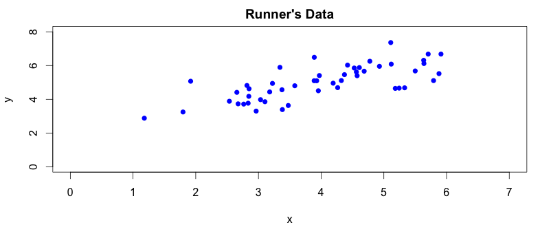
There are two things we can spot straight away from the plot. First, the camera angle is not perpendicular to the running track, so the collected data points are a bit rotated around the \(x\) axis. We can also notice, by drawing a simple regression line over the plotted data points, that there is a clear correlation between \(x\) and \(y\) coordinates captured by our camera:
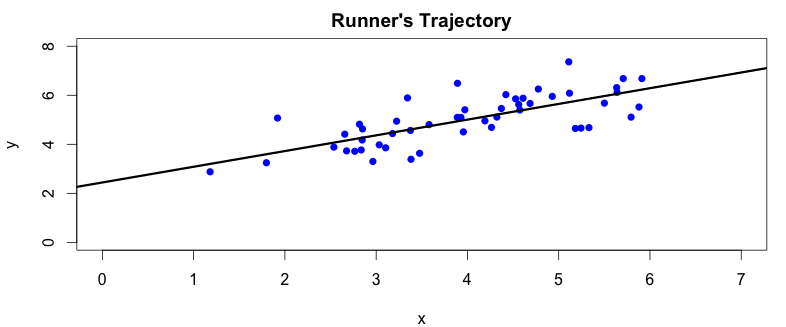
We should be able to figure out the parameters of the regression line from the captured data. This would allow us to calculate \(y\) from \(x\) and vice versa with some reasonable precision. Now we can see that our data set contains redundant information which does not provide any benefit. A single data point per measurement should be enough to describe the run. We will now try to use the PCA algorithm to identify and remove these data redundancies.
You can find the source code to the above plots in my GitHub repo
Problem definition
Now that we are hopefully a bit more familiar with the practical issues PCA tries to solve, we will try to formalize them as a mathematical problem. Once we find a solution to this problem, we will codify it in our favourite programming language. Many Machine Learning algorithms require some knowledge of Linear algebra, Calculus and Statistics. PCA is no different. This article assumes the reader has at least basic understanding of the above listed topics.
We will start by expressing the measured data as a matrix \(X\). Each row of the matrix \(X\) will hold a separate pair of measured coordinates. The matrix will have 50 rows (one row per measurement) and 2 columns (one column for each coordinate). You can see the first few rows of matrix \(X\) below:
$$ X = \left[\begin{array} {rrr} 3.381563 & 3.389113 \\ 4.527875 & 5.854178 \\ 2.655682 & 4.411995 \\ \vdots & \vdots \end{array}\right] $$
We know from linear algebra that each pair of coordinates our camera captured represents a two dimensional vector which lies in some vector space of the same dimension. We also know that any vector space is defined by its vector basis, sometimes called vector space generators. Vector space basis is a maximal set of linearly independent vectors that can generate the whole vector space via their linear combination. Put another way: every vector in particular vector space can be expressed as a linear combination of the vector space basis.
Let’s consider some basic two dimensional basis vectors \(b1\) and \(b2\). Let us further assume \(b1\) and \(b2\) comprise othornormal basis. We will now lay them into some matrix \(B\) by columns:
$$ B = \left[\begin{array} {cc} b1 \\ b2 \end{array}\right] = \left[\begin{array} {cc} 1 & 0 \\ 0 & 1 \end{array}\right] $$
We can express the first measurement in matrix \(X\) using this basis like this:
$$ x_1 = \left[\begin{array}{cc} 3.381563 & 3.389113 \end{array}\right] = 3.381563 * b1 + 3.389113 * b2$$
Every measurement in matrix \(X\) can be expressed using the same vector basis in a similar way. We can formalize this using a simple matrix equation:
$$ XB = X $$
It’s worth noting that expressing the data via the orthonormal basis does not transform it. This is an important property of orthogonal data projection - idempotency:
$$ XB = X = (XB)B $$
We now know that our measurements lie in the vector space defined by the vector basis \([b1, b2]\). The “problem” with the basic basis is that it is often not the best basis to express your data with. If we look at the plot we have drawn earlier we can see that the basic basis, which point in direction of the plot coordinate axis, is not in line with the camera angle from which we were recording the runner’s movement. If it were, the plotted data points would fluctuate around \(x\) axis pointing in the direction of the runner’s trajectory. The basic vector basis reflects the method we gathered the data, not the data itself!
Is there a different vector basis which is a linear combination of the basic basis that best expresses our data?
Answering this question is the goal of PCA. If such basis exists, expressing our data using this basis will transform (rotate) the original data in a way that describes it in a way that can highlight its important features. We can formalize this goal using the following matrix equation:
$$XB’= X’$$
where matrix \(X’\) contains the transformed data, matrix \(B’\) holds the new vector basis in its columns just like matrix \(B\) held the basic vector basis. If we look closely at this equation, we will notice that there is nothing surprising about it. It merely formalizes the data transformation using the new vector basis.
$$ XB’ = \left[\begin{array} {cc} x_1 \\ x_2 \\ \vdots \end{array}\right]\left[\begin{array} {cc} b’_1 & b’_2 & \ldots \end{array}\right] $$
$$ X’ = \left[\begin{array} {cc} x_1 * b’_1 & x_1 * b’_2 & \ldots \\ x_2 * b’_1 & x_2 * b’_2 & \ldots \\ \vdots & \vdots \end{array}\right] $$
Each row of matrix \(X’\) contains a particular data row of matrix \(X\) expressed in the new basis. It’s also worth pointing out that the idempotency property mentioned earlier still holds true on the transformed data:
$$X’B’ = X’ = (X’B’)B’$$
We have now formalised our goal to a search for a new vector basis that can re-express our original data different way. This new set of vector basis are the principal components we are looking for.
We still do not know based on what criterias do we choose the new basis. The answer to this question turns out to be quite simple: information. Put another way: the new vector basis should transform the original data in a way that retains as much information about the original data as possible.
Information retention
Our task is to find a data transformation that will retain as much information of the original data as possible. We can measure the information present in arbitrary data sets by a well known signal to noise ratio (SNR) defined as follows:
$$ SNR = \frac{\sigma^2_{signal}}{\sigma^2_{noise}} $$
where \(\sigma^2_{signal}\) and \(\sigma^2_{noise}\) represent the variances of signal and noise in the data set.
Variance is an important statistical measure which helps us understand spread of the data in a data set. It is defined as follows:
$$ var(X) = \frac{\sum_{i=1}^n(X_i - \overline{X})(X_i - \overline{X})}{(n-1)} = \frac{\sum_{i=1}^n(X_i - \overline{X})^2}{(n-1)} $$
where \(x\) is a vector of measurements, \(\overline{x}\) is its mean value and \(n\) is a number of data samples in vector \(X\).
From the \(SNR\) formula we can see that the higher the \(SNR\) the more signal there is available in the data. This means that in order to retain as much information from our original data, the new vector basis we are searching for, should point in the direction of the highest variance: the higher the variance the more information we retain. If we apply this intuition to the runner’s data, we should discover that the direction of the highest variance follows the trajectory of the runner’s movement.
Covariance matrix
Variance is a pretty good statistical measure, however it is only useful for single dimensional data i.e. vectors. It does not help when we are trying to find out if there is any relationship between any types of data features in arbitrary data sets. We need a better measure that will be able to capture these relationships. Covariance provides such measure. Covariance is always measured between two arbitrary data sets of the same length. It is defined as follows:
$$cov(X,Y) = \frac{\sum_{i=1}^n(X_i - \overline{X})(Y_i - \overline{Y})}{(n-1)}$$
where \(X\) and \(Y\) are two arbitrary vectors holding \(n\) number of measurements and \(\overline{X}\) and \(\overline{Y}\) are their mean values. You might have noticed that if we calculate covariance with the data itself, we will get the variance:
$$cov(X,X) = \frac{\sum_{i=1}^n(X_i - \overline{X})(X_i - \overline{X})}{(n-1)} = var(X)$$
So what does covariance actually tell us about two data sets? Its exact value is not actually as important as it is its sign:
- if the sign is positive, then both data sets increase together
- if the sign is negative, then both data sets decrease together
- if the covariance is zero, the two data sets are independent
According to tese properties two data sets are correlated ONLY IF their covariance is non-zero. If we now calculate the covariance between the two columns in the runner’s data matrix we will notice that the resulting value is positive. This confirms our suspicion about the relationship between the collected coordinates: our data set really is redundant.
Covariance is helpful when dealing with two dimensional data. But what if we are trying to figure out a possible relationship in data sets that span larger number of dimensions? We use covariance matrix which is defined as follows:
$$ C_X = \frac{1}{n}X^TX$$
where \(n\) is a number of rows (measurements) of matrix \(X\). Note that the data columns of matrix \(X\) have been “mean centered” as per the covariance formula! The importance of mean centering is discussed in several scientific papers – for the purpose of this article all of our data are mean centered [according to the definition of covariance].
Covariance matrix is extremely valuable as it carries the information about relationships between all measurements types stored in particular column vectors of our data matrix. This might not be obvious from the formula, so let’s have a look at a simple example to understand this better. Let’s consider a three dimesional data matrix (i.e. the matrix has 3 columns) to illustrate some important properties of the covariance matrix. The example data matrix \(Y\) will hold three different types of measurements in its column vectors \(x\), \(y\) and \(z\). Let’s also assume that data stored in each of these vectors have already been mean centered:
$$Y = \left[\begin{array} {cc} x & y & z \end{array}\right]$$
If we now calculate its covariance matrix \(C_Y\) we will get the following result:
$$ C_Y = \frac{1}{n}\left(\begin{array} {cc} x & y & z \end{array}\right)^T\left(\begin{array} {cc} x & y & z \end{array}\right) = \left(\begin{array} {cc} cov(x,x) & cov(x,y) & cov(x,z) \\ cov(y,x) & cov(y,y) & cov(y,z) \\ cov(z,x) & cov(z,y) & cov(z,z) \end{array}\right) $$
The properties of the covariance matrix should now be more obvious:
- covariance matrix is a square symmetric matrix of size \(n \times n\) where \(n\) is a number of data measurements
- diagonal terms are the variances of particular measurement types which carry the signal
- off-the diagnoal terms are the covariances between particular measurement types which signify the noise
We know that the bigger the variance, the higher the signal. We also know that non-zero covariance signifies the presence of the noise (in form of data redundancies). In light of this knowledge we can now rephrase our goal to finding a new vector basis which maximises variance and minimises covariance of the trasnformed data set features.
In the most idealistic scenario, we would like the PCA to find the new vector basis so that the covariance matrix of the transformed data is diagonal i.e. its off-the diagonal values are zero. There is one subtle assumption PCA makes about the new basis: the new vector basis is orthogonal. Orthogonality makes finding the new basis fairly easy task solvable with linear algebra. We will discuss this more in the next part of this series where we formalize the PCA algorithm in simpe steps.
Conclusion
In this blog post we have laid down the most important knowledge bricks for understanding Principal Component Analysis. We learnt that the PCA tries to find a new vector basis that transforms the original data to a new data set in a way that maximizes variances of particular measurement types and at the same time minimizes covariances between them.
The new vector basis points in a direction of the highest variances. Orthogonality of the new vector basis assumption puts a restriction on the basis direction: imagine playing an old arcade game like pacman where you can only move your character in direction of right angles.
In the next part of this series we will look into the actual implementation of PCA. We will then apply it to our simple two dimensional example of runner’s data. Finally we will look at more complex multidimensional data like digital images and show a simple data compression algorithms based on PCA.
Acknowledgements: Thanks to Kushal Pisavadia for reading the first draft of this post and providing valuable feedback.